The basis of this post is the inTrees (interpretable trees) package in R [CRAN].  The inTrees package summarizes the typically complex result of tree based ensemble learners/algorithms into rule-based learners referred to as Simplified Tree Ensemble Learner (STEL). This approach solves the following problem: Tree based ensemble learners, such as RandomForest (RF) and Gradient Boosting Machines (GBM), often deliver superior predictive results compare to more simple decision tree or other low complexity models, but are difficult to interpret or offer insight. I will use an archaeological example here (because my blog title mandates it), but this package/method can be applied to any domain.

Oh Archaeology… We need to talk:

Ok, let’s get real here.  Archaeology has an illogical and unhealthy repugnance to predictive modeling. IMHO, illogical because the vast majority of archaeological thought process are based on empirically derived patterns based on from previous observation.  All we do is predict based on what data we know (a.k.a. predict from models, a.k.a. predictive modeling). Unhealthy, because it stifles creative thought, advancement of knowledge, and relevance of the field.  Why is this condition so?  Again, IMHO, because archaeologists are stuck in the past (no pun intended), feel the need to cling to images of self-sufficient site-based discovery, have little impetus to change , and would rather stick to our area of research then coalesce to help solve real-world problems. But, what the hell do I know.

What the heck does this have to do with tree based statistical learning?  Nothing and everything.  In no direct sense do these two things overlap, but indirectly, the methods I am discussing here have (once again) IMHO, the potential to bridge the gap between complex multidimensional modeling and practical archaeological decision making.  Further, not only do I think this is true for archaeology, but likely for other fields that have significant stalwart factions.  That is a bold claim for sure, but having navigated this boundary for 20 years, I am really excited about the potential for this method; more so than most any other.

Bottom lines is that the method discussed below, interpretable trees from rule-based learners in the inTrees package for R, allows for the derivation of simple-to-interpret rule based decision making based on empirically derived complex and difficult-to-interpret tree based statistical learning methods.  Or more generally, use fancy-pants models to make simple rules that even the most skeptical archaeologist will have to reason with.  Please follow me…

Trees, Ensembles, and Rule-based Learners

The inTree methodology goes a long way to solving the problem posed at the opening of this post.  The strength of ensemble tree models, variance reduction through aggregation, is also the source of weakness for interpretation.  Ensemble models are made of numerous, tens to tens of thousands of single tree models, that on their own are easy to interpret (as we will see).  However an ensemble model is created from the collective “forest” of individual tree models, from which predictions are taken from a consensus of the forest.  The ensemble method reduces the individual fluctuations in single tree models (variance) through averaging over the variance of many models.  Although, as we average over the forest of models, we lose the easy to interpret rules of each individual model.  InTrees seeks to re-establish the simplicity of individual rules while retaining the lower variance predictions of the forest; a very noble goal.

Wait, remind me again why this is about archaeology?  Briefly, because while archaeologists have very little experience or trust in ensemble based learners, they are pretty comfortable discussing classification based on the logic of decision trees.  The inTrees methods allows for the construction of ensemble models that are presented as simple rule based systems that are able to more easily penetrate the policy of a reluctant archaeologist or agency. If the simple rule model can be shown to be as effective or nearly as effective as the ensemble model and roughly congruent with experienced based mental models, then it is a win/win/win for everyone.

Decision Trees; the Basics

At the atomic level, a decision tree is composed of a single data based decision that branches to two results based on either a binary “yes” or “no” or a threshold value (i.e. greater than 100 and less then 100).  The simple form of one decision and two results is called a decision stump. The tree metaphor is pretty obvious in the dendritic branching structure.  The results at the bottom of the [inverted] tree are called leaf nodes. In the leaf nodes can non-exclusivley contain the count of observations that fall meet the trees criteria or a probability of class resulting in that node.  These are incredibly flexible data structures and very applicable to many modeling/classification problems. All of the following example tress are totally fictitious and not based on real data.

 

The decision stump is then expanded into a tree as new decision nodes are added.  A shallow tree is one with few branching nodes, a deep tree has many nodes, and a fully grown tree continues to add nodes until each data point [observation] is classified into its own individual leaf node.

Finally, this logical structure is clear formalization of how most archaeologists’ think and are taught to think about the potential for site location in unsurveyed areas.  “Is the location near water?”; “Is the slope moderate to low?”; “Is there a source of high quality lithic material near by?”.  These are all questions that will likely go through an archaeologists head, adjusted for their local constraints, when the sensitivity of any unsurveyed are is considered.  The formalization of that approach in the tree structure is simple to see.  Here is an environmentally based tree that may be applicable to pre-contact sites, but substitute distance to historic road, presence of mineral resources, availability of navigable waterway, or the like for a historic model.

Now the point of this post is to show how we expand this simple model into a data based ensemble of many trees to achieve potentially much better predictive results.

Tree Ensembles….

The problem with single decision trees in the context prediction is that they can look very different as new samples of data are applied.  Take 10 observations (site locations) and build a tree.  It may fit that data very well, but predict other sites very poorly.  Fit the same tree with 10 new observations and the tree may look very different and predict other sites very differently.  This is called a model having high variance and that is typically a bad thing.  The idea behind ensembles is the reduction of variance by building many, tens to tens of thousands, of individual trees and then predicting based on the consensus of all those trees.  In some common forms, that consensus is taken as the decision of a majority of the trees.  There are many specific ensemble algorithms, including varieties of Random Forests and varieties of Gradient Boosting, but most any model can be ensembled to reduce individual model variance.  Basically, as we increase the number of models in the ensemble, the variance is divided by at a rate controlled by the correlation of each model.  The lower the correlation in the models, the greater the reduction of variance. Ensemble algorithms are deigned to take advantage of this feature to produce very good predictive results that can have both low bias and low variance if tuned correctly.  I have touched on the concept of the bias/variance tradeoff here and there, but others do it much better, here, here, and definitely here.

The problem with Ensembles…

The problem with an ensemble, be it three thousand decision trees or three completely different models stacked, is that the ease of interpretation of a single model is lost.  If we fit a set of site location data across a forest or decision trees, the variance between trees will make it very difficult to try to find a single thread of common decision between them.  Fortunately, that is difficult, not impossible.  Truthfully, in many settings the interpretability of a simple model is not as important as an objectively low prediction error.  In those settings, if the model works well against some predefined benchmark, then the why it works is not important; as long as it works.  In other settings, the why can be equally if not more important that optimizing a model for the lowest possible prediction error.  I’d argue that in archaeology very often the why a model works is critical in getting stakeholders or policy makers to agree on an implementation; even if optimizing prediction accuracy is the stated model goal.

The inTrees solution…

In most modeling context, the interpretability of a model and a model’s ability to reduce variance [generally improving prediction] are often on opposite sides of the spectrum.  The ability to close this gap would allow for both model interpretability in addition to reduced variance and better model prediction.  The inTrees package has a method to do just that.  The results presented below show that in these tests, the inTrees method can match, if not improve upon, the performance of the complex ensemble models while offering interpretable results.  This is a very powerful thing.

How does inTrees work…

The inTrees package works by taken a tree based ensemble fit to your data, extracting the rules that govern the splits in each of the ensembles trees (may be in the thousands), compares these rules to the true class label [y/dependent variable], processes these rules by removing duplicates, measuring rule length, and pruning rules down to their simple form, and finally these processed rules are summarized into a simple set of if/then rules.  This in known as a simplified Tree Ensemble Learner (STEL)  The STEL of the in/then rules can then be used as-is for real world decision making or applied to new data as a simple model for prediction/classification.  The former use of a real world decision making tool is what I have been espousing thus far in the post and is a great reason to use this approach.  However, the latter reason of a new model is really interesting and powerful; I will continue to explore this.  The author of the inTrees package, Houtao Deng, has written a great paper explaining the approach and has a website with updated info.

The power of this is that the STEL is just a basic if/then statements in plain text and therefore can be implemented in any programming language and run at speed and scale.  An example scenario is fitting your Random Forest of GBM model in R [what else would you use?], which may take minutes to hours to fit.  But you want to implement this model as a simple web-form so after going through the inTrees method you implement the simple STEL rules in JavaScript of PHP even and it runs instantly.  This negates the need for an R server running in the background and the overhead of processing, prediction, and translation back to the web.  This begs the question: “How does the performance of the STEL classification compare to the original ensemble?”  A great question.  The answer will depend on how important model interpretability or language-agnostic implementation is to you, but in my examples presented below, the performance of the STEL is very comparable to the original ensemble from which it is derived.

An Example; Rules, Prune, STEL

Lets look at an example. I start by taking a dataset of 6828 observation of points within 200 archaeological sites in a single physiographic provence and splitting it into 75% training data and 25% testing data.  The test/train split makes sure the observations from a single site are only within either test or train; this reduces the spatial correlation of samples to at least the inter-site level.  This data set is reduced to only three variables to save on time and add simplicity.  These are the minimum Euclidian distance to a water source [e_hyd_min], the standard deviation of slope within a 32 cell neighborhood [std_32c], and the change in elevation from any cell to the head of a stream drainage [elev_2_drainh].  I create a test dataset called dat_rnd that is a rounded version of the raw measurements.  The class label here is call presence and is a binary 0/1 indicating the absence or a site or presence of a known site respectively.  The final line chops the testing data down to the same variables.

train <- test_train[["train"]]
test <- test_train[["test"]]
dat_rnd <- data.frame(e_hyd_min = round(train$e_hyd_min,1),
std_32c = round(train$std_32c,2),
elev_2_drainh = round(train$elev_2_drainh,2))
target <- as.factor(train$presence)
test_learned <- test[,c("e_hyd_min", "std_32c", "elev_2_drainh", "presence")]

The next code block is the implementation of the inTrees method.  First I fit a basic Random Forest model on the training dataset [dat_rnd]. We make a a rules list as treelist, we extract the rules as exec, get, prune, and select the best rules as ruleMetric,  build a STEL learner as learner, and finally recompose the learner into a set of readable rules as Simp_Learner.  The learner is plenty readable, but Simp_Learner replaces the column index with actual column names so the variables can be read without having to be looked up.

 rf <- randomForest(dat_rnd, target)
treeList <- RF2List(rf) # transform rf object to an inTrees' format
exec <- extractRules(treeList,dat_rnd) # R-executable conditions
ruleMetric <- getRuleMetric(exec,dat_rnd,target) # get rule metrics
ruleMetric <- pruneRule(ruleMetric,dat_rnd,target)
ruleMetric <- selectRuleRRF(ruleMetric,dat_rnd,target)
learner <- buildLearner(ruleMetric,dat_rnd,target)
Simp_Learner <- presentRules(ruleMetric,colnames(dat_rnd))

The STEL that results from the original RF model [default 500 individual trees], looks like this:

Rule	Length	Frequency	Pred Err.	Condition	Pred Class	impRRF
1	2	0.412	0.25	e_hyd_min>162.5 & std_32c<=22.13	0	1.00
2	4	0.142	0.08	e_hyd_min<=77.05 & std_32c>7.73 & std_32c<=16.065 & elev_2_drainh<=-3.5	1	0.27
3	2	0.321	0.21	e_hyd_min>205.55 & elev_2_drainh<=59.5	0	0.14
4	3	0.062	0.23	std_32c>4.745 & std_32c<=5.445 & elev_2_drainh<=-2.5	1	0.12
5	3	0.401	0.35	std_32c<=6.945 & std_32c>1.925 & elev_2_drainh>-10.5	0	0.11
6	2	0.023	0.06	std_32c<=24.06 & std_32c>16.23	0	0.07
7	3	0.016	0.41	e_hyd_min>5.3 & e_hyd_min<=18.15 & elev_2_drainh>-12.5	0	0.02
8	2	0.055	0.53	e_hyd_min<=31 & std_32c<=9.13	0	0.01

This table is the STEL that distills a forest of 500 trees into the sort of simple decision rules that are easily interpreted and easily applied to new observations.  For each rule [row] we get the length of the rule, as in the number of decisions per rule; the frequency of that rule appearing in the forest, the prediction error of that rule, the rule itself, the class [presence = 1 / absence = 0] predicted by that rule and a measure of each rules relative importance in predicting the correct class. [*Note: this is not totally true as the impRFF measures the percent relative decrease in Gini index (node purity) for each rule derived from a Regularized Random Forest (RRF) fit to the rule set and regularized by the the length of each rule as a proxy for rule complexity.  It took a bit of research to get to this understanding of how inTrees implements impRRF, but it is beyond the scope of this post.]

Following this table, the most important rule for detecting non-site/background areas is described as e_hyd_min > 162.5 & std_32c <= 22.13, read as greater than 162.5 meters from any water source and a standard deviation of percent slope over a ~320-meter neighborhood of less than or equal to 22.13.  Since a  STD of slope of less than 22.13 is a darn high range of slopes and covers a lot of ground here, it is the distance from water that is likely most important.  This rule has a frequency of 41.2% and a impRRF of 1, so it is a common and important rule.  The prediction error rate is 25%, which is pretty darn high, but the other metrics suggest it is broadly applicable and general.

The most important rule for predicting site presence is described as e_hyd_min <= 77.05 & std_32c > 7.73 & std_32c <= 16.065 & elev_2_drainh <= -3.5, and read as site presence is predicted at locations that are less than or equal to 77.05 meter from a water source, a standard deviation of slope of less than or equal to 16.06, and at areas slightly higher higher in elevation that drainage heads.  This rule covers 13.2% of sites in the training sample with a prediction error of 8%.  This rule is applicable to a relatively broad section of known site samples and has a relatively low error rate.  The other rule that was selected to predict site presence is described as std_32c > 4.745 & std_32c <= 5.445 & elev_2_drainh <= -2.5, low variation os slope between 4.7 and 5.4 standard deviations and above drainage heads.  This site presence rule has a lower frequency and higher error rate than the previous, but is somewhat discriminatory (in the world of archaeological predictive models). The rest of the rules describe various segments of non-site predictions.

The long and short of this post is that this STEL is a super simple and interpretable set of rules that any human and interpret and predict from.  If you have a new area to look at, calculate these variable values (likely requiring a GIS) and filter them through the rule set; thats all.  This represents a complex ensemble of 500 trees distilled into a STEL of 8 rules and accompanying frequency, prediction error, and importance measures.  Pretty damn cool.

Model comparison

The above code was repeated for a series of different algorithms that include RF, GBM, and Recursive Partitioning (rpart).  These are all tree based methods with rpart being the most basic and based on a single tree.  RF, mentioned above, is an ensemble of many trees that uses bagging to bootstrap groups of data for each tree and randomly selects variables to try at each decision split.  Finally, GBM is a boosting method that is also an ensemble, but uses tree stumps to make weakly predictive trees and then integrates over the results to work harder on fixing the prediction errors from the previous round. This is totally hand-wavy, but this is not the place to deep-dive on these algorithms.  Just google them and you will get a host of great descriptions.  The important part is that they are all tree based methods and can be implemented in the inTrees package to derive a STEL.

For each of RF, rpart, and GBM, I ran each model 20 times using randomly selected and split site samples with 75% training and 25% testing. The full site sample is 200 sites in the same physiographic section.  After the RF and GBM models were fit, I predicted the testing site sample using both the original fit model and the STEL derived from the fit model using the inTrees method in the code above. The rpart model is only a single tree and not an ensemble, so there is no STEL to be had here.

The results of this will give not only the relative prediction error of each different algorithm on this data set, but also the comparison of the simple rule based STEL prediction versus the prediction method inherent to each algorithm.  Have an acceptable similar prediction error between the STEL and inherent prediction method would go a ways to justify the use of the simplified rules because they are interpretable, easily implemented, and do not sacrifice a significant amount of predictive power… if you are into those sorts of things.

Comparing Models vs. STEL

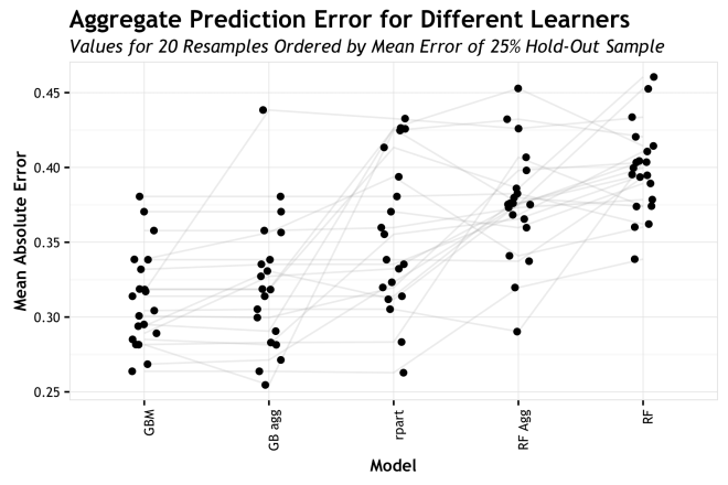
The graphic below shows the prediction results of the 20 iterations across randomly split datasets for three different models and two different prediction methods (STEL and inherent).  The x-axis is ordered by increasing mean prediction error per algorithm/prediction method across the 20 model runs.  The STEL versions of the RF and GBM models have the suffix “agg” because they are the aggregate of the ensemble. The light gray lines connect each of the models for each of the 20 runs.  This is not a crucial piece of info, but it helps visualize how consistent each model ranks given a randomly spit dataset. The y-axis is the Mean Absolute Error of each model run (MAE).

In this test, GBM has the lowest mean prediction error across all runs, the the lowest absolute error cam from predicting the STEL of the GBM. the basic rpart model in the middle of the tested algorithms, but also has the largest variance in MAE.  For the RF algorithm, the STEL version has the lower mean MAE, but greater variance than the inherent prediction method for RF.  So, in all, the simple rpart model has the highest variance, which fits because that algorithm does not use the variance reducing methods of the other ensembles.GBM and the STEL of GBM (GBM agg) have the lowest mean MAE and in my experience GBM and XGBM are often superior in predictive performance to other algorithms.  Finally, in general, the STEL prediction has equal if not better mean MAE across the 20 samples, but in both cases higher variance; also not entirely surprising.  It is comforting to see that the MAE of the STEL is not significantly worse that the inherent prediction method.  At least for this data set, this would make me comfortable in presenting the STEL as the simple interpretation of the data and then if it made sense in the larger archaeological context, predicting based upon it.

Tabular results and medians per model and randomized data split are presented here:

Run	RF.Agg	GB.agg	rpart	RF	GBM	Median
1	0.47	0.36	0.35	0.40	0.50	0.44
2	0.41	0.36	0.41	0.41	0.35	0.41
3	0.41	0.40	0.40	0.40	0.41	0.40
4	0.41	0.38	0.35	0.43	0.31	0.39
5	0.39	0.26	0.31	0.43	0.26	0.35
6	0.35	0.36	0.36	0.35	0.48	0.36
7	0.35	0.35	0.35	0.41	0.35	0.35
8	0.30	0.28	0.30	0.33	0.29	0.30
9	0.41	0.41	0.42	0.42	0.45	0.42
10	0.32	0.34	0.33	0.36	0.33	0.33
Median	0.40	0.36	0.35	0.41	0.35	0.38

Conclusion

The conclusion is that the inTrees package gives a great method for deriving simple rule based learners from complex tree based ensembles.  Better yet, the predictive results are roughly as good, albeit probably higher variance compared to the inherent prediction methods of the RF and GBM algorithms.  Better yet, the simplified rules based STEL can be implemented in any programming language or via pen and paper (and a little patience).  Be it archaeological site locations, high blood pressure warnings, or credit card fraud, the STEL offers the an intuitive way to communicate a complex ensemble model to anyone. In my experience, getting  getting people to buy into a model and explore deeper than the fancy-numbers-and-maps factor is the real challenge of this enterprise.  The inTrees method is a huge step in that direction.

Notes:

The code for the simulation over all models is located in this GIST

> sessionInfo()
R version 3.2.2 (2015-08-14)
Platform: x86_64-apple-darwin13.4.0 (64-bit)
Running under: OS X 10.10.5 (Yosemite)

locale:
[1] en_US.UTF-8/en_US.UTF-8/en_US.UTF-8/C/en_US.UTF-8/en_US.UTF-8

attached base packages:
[1] parallel splines stats graphics grDevices utils datasets methods base

other attached packages:
[1] scatterplot3d_0.3-37 ggalt_0.3.0.9000 reshape2_1.4.1 rpart_4.1-10
[5] gbm_2.1.1 survival_2.38-3 caret_6.0-64 ggplot2_2.1.0
[9] lattice_0.20-33 xtable_1.8-2 randomForest_4.6-10 inTrees_1.1
[13] rowr_1.1.2 data.table_1.9.4 dplyr_0.5.0

loaded via a namespace (and not attached):
[1] colorspace_1.2-6 stats4_3.2.2 mgcv_1.8-11 chron_2.3-47 nloptr_1.0.4
[6] DBI_0.4-1 RColorBrewer_1.1-2 foreach_1.4.2 plyr_1.8.4 stringr_1.0.0
[11] MatrixModels_0.4-1 munsell_0.4.3 gtable_0.2.0 codetools_0.2-14 SparseM_1.7
[16] extrafont_0.17 quantreg_5.19 pbkrtest_0.4-2 Rttf2pt1_1.3.4 RRF_1.6
[21] Rcpp_0.12.5 KernSmooth_2.23-15 scales_0.4.0 jsonlite_1.0 lme4_1.1-9
[26] proj4_1.0-8 stringi_1.1.1 ash_1.0-15 grid_3.2.2 tools_3.2.2
[31] magrittr_1.5 arules_1.4-1 maps_3.1.0 lazyeval_0.2.0 tibble_1.0
[36] extrafontdb_1.0 car_2.1-0 MASS_7.3-43 Matrix_1.2-2 rsconnect_0.4.1.4
[41] assertthat_0.1 minqa_1.2.4 iterators_1.0.7 R6_2.1.2 nnet_7.3-10
[46] nlme_3.1-121
>