Gaussian Process Hyperparameter Estimation

~~Quick~~ Way longer then expected post and some code for looking into the estimation of kernel hyperparameters using STAN HMC/MCMC and R. I wanted to drop this work here for safe keeping. Partially for the exercise of thinking it through and writing it down, but also because it my be useful to someone. I wrote a little about GP in a previous post, but my understanding is rather pedestrian, so these explorations help. In general GPs are non-linear regression machines that utilize a kernel to reproject your data into a larger dimensional space in order to represent and better approximate the function we are targeting. Then using a covariance matrix calculated from that kernel, a multivariate Gaussian posterior is derived. The posterior can then be used for all of the great things that Bayesian analysis can do with a posterior.

Read lots more about GP here…. Big thanks to James Keirstead for blogging a bunch of the code that I used under the hood here and thanks to Bob Carpenter (github code) and the Stan team for great software with top-notch documentation.

code:

The R code for all analysis and plots can be found in a gist here, as well as the three Stan model codes, here gp-sim_SE.stan, gp-predict_SE.stan,and GP_estimate_eta_rho_SE.stan

sin2_header

The hyperparameters of topic here are parameters of the kernel within the GP algorithm. As with other algorithms that use kernels, a number of functions can be used based on the type of generative function you are approximating. The most commonly used kernel function for GP (and seemingly Support Vector Machines) is the Squared Exponential (SE), also known as the Radial Basis Function (RBF), Gaussian, or Exponentiated Quadratic function.

The Squared Exponential Kernel

The SE kernel is a negative length scale factor rho ( $\rho^2$ ) times the square distance between data points ( $(x -x^\prime)^2$ ) all multiplied by a scale factor eta ( $\eta$ ). Rho is a shorthand for the length scale which is often written as a denominator as shown below. Eta is a scale factor that determines how far the function varies from the mean. Finally sigma squared ( $sigma^2_{noise}$ ) at the end is the value for the diagonal elements of the matrix where ( $i = j$ ). This last term is not necessarily part of the kernel, but is instead a jitter term to set zero to near zero for numeric reasons. The matrix created by this function is positive semi-definite and composed of the distance between observations scaled by rho and eta. Many other kernels (linear, periodic, linear * periodic, etc…) can be used here; see the kernel cookbook for examples.

$k_{x,x^\prime}=\eta^2 \exp(-\rho^2 (x -x^\prime)^2)+\delta_{ij}\sigma^2_{noise} \\ \rho^2 = 1/(2\ell^2) \\ \delta_{ij}\sigma^2_{noise}=0.0001$

To Fix or to Estimate?

In this post, models are created where $sigma^2_{noise}$ , $\rho^2$ , and $\eta^2$ are all fixed, as well as a model where $sigma^2_{noise}$ is fixed and $\rho^2$ and $\eta^2$ are free. In the MCMC probabilistic framework, we can fix $\rho^2$ and $\eta^2$ or any parameter for the most part, or estimate them. To this point, there was a very informative and interesting discussion on stan-users mailing list about why you might want to estimate the SE kernel hyperparameters. The discussion generally broke across the lines of A) you don’t need to estimate these, just use relatively informative priors based on your domain knowledge, and B) of course you want to estimate these because you may be missing a large chunk of function space and uncertainty if you do not. The conclusion to the thread is a hedge to try it both ways, but there are great bits of info it there regardless.

So while the greatest minds in Hamiltonian Monte Carlo chat about it, I am going to just naively work on the Stan code to do these estimations and see where it takes me. Even if fixed with informative priors is the way to go, I at least want to know how to write/execute the model that estimates them. So here we go.

The SE Kernel Prior

The SE kernel is the scale factor $\eta^2$ times the exponentiated product of negative $\rho^2$ and squared distance of $x_i$ and $x_j$ ; for indices i and j where i = j = length(x). Sigma is an i by j matrix. Below are a few different ways this kernel can be written in R; 1) the simple code way with rho times the squared distance; 2) as often written formally with $2\ell^2$ as the length parameter; and 3) an intermediate way with the squared distance divided by the inverse of rho. As far as relating $\ell$ and $\rho^2$ , $\rho^2 = \frac{1}{2\ell^2}$ and $\ell = \sqrt{\frac{1/\rho^2}{2}}$

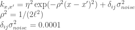
    ## Simplified form
    Sigma[i,j] <- eta_sq * exp(-rho_sq*(x[i] - x[j])^2) +
    ifelse(i==j, sigma_sq, 0.0)
    ## Length parameter == l instead of rho_sq
    Sigma[i,j] <- eta_sq * exp(-((x[i] - x[j])^2)/(2*(l^2))) +
    ifelse(i==j, sigma_sq, 0.0)
    ## Intermediate with rho_sq inplace of (2*l^2)
    Sigma[i,j] <- eta_sq * exp(-((x[i] - x[j])^2)/(1/rho_sq)) +
    ifelse(i==j, sigma_sq, 0.0)

Fortunately, it is simple to go from R to Stan in this instance. The differences are that ifelse() in R is if_else() in Stan and that we have to use the pow() function in Stan over the caret (^) operator in R.

    // simplified form
    Sigma[i,j] <- eta_sq * exp(-rho_sq*pow(x[i] - x[j],2)) +
    if_else(i==j, sigma_sq, 0.0)
    // Length parameter == l instead of rho_sq
    Sigma[i,j] <- eta_sq * exp(-((pow(x[i] - x[j],2))/(2*pow(l,2)))) +
    if_else(i==j, sigma_sq, 0.0)
    // Intermediate with rho_sq inplace of (2*l^2)
    Sigma[i,j] <- eta_sq * exp(-((pow(x[i] - x[j],2))/(1/rho_sq))) +
    if_else(i==j, sigma_sq, 0.0);

When this kernel is computed for a series of x, in this case x = seq(-5, 5, 0.05), we get a 201 x 201 matrix with identical upper and lower triangles. The diagonal where $D_{ij} =$ the variance $+ sigma^2_{noise}$ . The off diagonal is the covariance of $D_{ij}$ . The image below is a plot of matrix values using the lattice::levelplot() function.

Looking a little further, the $\rho^2$ parameter can be viewed as the inverse fall-off rate of correlation from the diagonal elements. The $\eta^2$ parameter is an overall scale parameter, so the graphic below looks essentially the same for all values of of $\eta^2$ relative to $\rho^2$ . As is evident, the high values along the diagonal fall off more quickly as the value of $rho^2$ increases. The intuition is that for the lower values of $\rho^2$ the kernel falls of slowly and relatively distant values are considered somewhat related. At the high end of $\rho^2$ , unless the values of very close, they have almost no relationship. If we were comparing the geographic distance of archaeological sites or features: for $\rho^2 = 0.01$ sites that were far apart would still have consequence on each other, where as at the other end, unless a site was directly proximal to another, they would have no influence on each other.

Put pretty generally (and hand-wavyey) that is how the kernel works. It computes a function based on the distance between $x_{ij}$ in the one dimensional space, or $x_{ij}y_{ij}$ in the two dimensional space (potentially anisotropic geographic space). The computation of this function over all $x_{ij}$ leads to a symmetric matrix defining the relationship between any two points in the data set. This is the matrix that defines the $\Sigma$ parameter of the multivariate normal distribution $MVN((0,\dots,0), \Sigma)$ from which the GP samples are drawn. There are many different ways to compute a kernel. Also, there are ways to combine (add, multiply) kernels. The SE kernel used here is the most commonly used and is very effective for a variety of problems.

The Gaussian Process

The GP is a Bayesian method and as such, there is a prior, there is data, and there is a posterior that is the prior conditioned on the data. In this example the kernel function and values of $\rho^2$ , $\eta^2$ , and $sigma^2_{noise}$ define the form of the prior along the x axis index. Samples of the prior can be simulated from a multivariate normal distribution where $y \sim MVN(\mu, \Sigma)$ ; $\mu$ = 0 and $\Sigma$ is our calculated kernel matrix. Below is a plot with 125 draws from our SE kernel parametrized by $\rho^2$ = 1, $\eta^2$ = 1, and $sigma^2_{noise}$ = 0.0001.

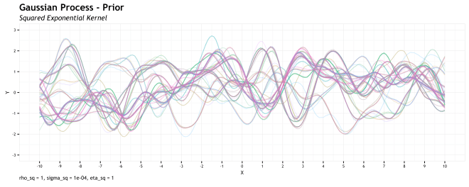
The above plot shows the logical implications of drawing functions from the multivariate Gaussian based on the kernel hyperparameter selection. This is not conditioned on data and therefore represents our prior assumption of the function space from which the data may be generated. Ok, so lets add some data…

RBF_data_example

Here I have 8 completely arbitrary data points that I made up. The bias behind these is that I wanted a somewhat evenly space set of $x$ coordinates and a somewhat periodically increasing set of $y$ values. I also wanted a bit of no-data space to the left to see how the functions operated in the absence of data. So, the goal here is to condition our prior assumptions on data to derive a posterior. We do this via HMC sampling using the Rstan package.

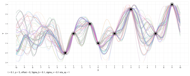
The graphic above shows the outcome of this process; the logical implications of conditioning our prior assumptions (based on kernel hyperparameters) on data. Since we are working under the assumption of noiseless data points (not very realistic), the functions of the posterior are those that pass through the data points. However, between data points, our uncertainty is expressed as variations in the function. To the left of the first data point, the model is pretty uncertain as to what the value of $y$ should be; our prior assumptions are most evident. In between data points, the flexibility of our functions (based to a large degree on $\rho^2$ ) governs the range of interpolations. Where data points follow a path that is inline with the kernel length scale hyperparameter (e.g. points 1 and 2, as well as 3 and 4), the model is more certain as to the interpolation. Conversely, the model is much less certain about the space between other data points (e.g. 6 and 7). The end result is a posterior distribution of functions from which we can infer the expectation and uncertainty. Granted, the first 20 times I heard that GP’s were a “distribution over functions.” I was like what in the heck are you talking about!? It became more clear as I toiled.

A more formal specification of the above model is as such:

$y \sim MVN((0, \dots, 0), K) \\ K =\eta^2 \exp(-\rho^2 D^2_{ij})+\delta_{ij}(0.0001) \\ \eta^2 = 1 \\ \rho^2 = 1$

How the prior effects our model

I went through all this kernel bit and what does it have to do with the GP? Essentially, the hyperparameters within the kernel affect various aspects of the resulting prior functions. On an abstracted level, they guide the kernel into properly encoding our assumptions about the functions into the matrix $\Sigma$ . In the case of the SE kernel, $\rho^2$ and $\eta^2$ control the length scale and magnitude, respectively, of the prior. Let’s see what happens when these are varied…

GP_SE_fitted_range_rho_eta_facet

This graphic pretty clearly illustrates what varying SE kernel hyperparameters does to the prior. Increasing $eta^2$ (moving from left to right) increases the amplitude of the wiggles in the function. Increasing $\rho^2$ (moving from top to bottom) decreases the periodicity of the wiggles in the function (remember, $\rho^2$ ) is an inverse of the length scale). Clearly $\rho^2 = 10$ , $\eta^2 = 10$ is a prior over very chaotic functions, where as $\rho^2 = 10$ , $\eta^2 = 10$ is a very mellow set of functions. Which is the correct set of parameterizations? Well, that is the main question of this ultra-long winded post.

Fitting this range of priors to our 8 data points, and we get the posteriors shown above. The combination of $\rho^2 = 0.1, \eta^2 = 0.1$ leads to a really pleasing set of gentle functions that pretty well approximate the periodic nature of the points as I envisioned them. Whereas $\rho^2 = 10, \eta^2 = 10$ is again chaotic. I find $\rho^2 = 10, \eta^2 = 0.1$ very interesting. This to me looks like an outlier detection function where a wide range of mean values are in the high probability region, but the functions have the amplitude flexibility to jump out and grab outlier when needed. Version in between the extremes have various levels of flexibility that lead to interesting patterns. Which posterior best fits the data? That depends entirely on the questions you are trying to answer and your favorite loss function.

Just for fun, I plotted the posteriors (purple) over the priors (orange) to see how they compare.

GP Kernel Hyperparameter Estimation

If you made it this far, you are a champ! So, which is the right set of hyperparameter values? If your prior knowledge or intuition does not give you this answer, you can use sampling to help figure it out. With the stan/HMC/MCMC framework, we can specify the random variables of the model that we want to estimate. As good Bayesians, we are rewarded with a distribution over that random variable and then we can infer from it. In this case, I am interested in estimating both $\rho^2$ and $\eta^2$ conditioned on my data. The Stan code here does such. A formalization of this model include the HalfCauchy(0,5) priors over the $\rho^2$ and $\eta^2$ hyperparameters. The choice of HalfCauchy(0,5) is an subjective choice of both a distribution and a subsequent set of center and scale hyperparameters; parameters that could also be sampled and estimated… But in this case, it is a relatively weakly-informative prior that regularizes of random variables of interest. Note that in the stat code it is a cauchy(), but is defined as real<lower=0> to confine the distribution to positive reals and has a location parameter of zero.

$y \sim MVN((0, \dots, 0), K) \\ K =\eta^2 \exp(-\rho^2 D^2_{ij})+\delta_{ij}(0.0001) \\ \eta^2 = HalfCauchy(0, 5) \\ \rho^2 = HalfCauchy(0, 5)$

To visualize the results in a similar manner as before, we must choose values from the resulting distributions of $\rho^2$ and $\eta^2$ and apply our model. The graphic below shows the posterior for a range of values. At the top, the 5% value for both $\rho^2$ and $\eta^2$ are taken jointly. Similarly, the median (50%) is the middle facet, and the 95th percentile (high) of the hyperparameter distribution is the lower plot. These three plots show the posterior for the 5% to 95% parameter estimation for both $\rho^2$ and $\eta^2$ jointly. Notice that the HMC sampling did not result in the chaotic functions of the previous plots.

So, the posterior for the joint hyperparameter estimation is interesting, but what about when they are combined for the range of the distribution? As above, low = 5%, median = 50%, and high = 95%. In the below plot, the left to right diagonal is the same hyperparameter combinations as the above plot. The upper right shows the 95th percentile scale (amplitude) hyperparameter with the 5th percentile inverse length scale parameter. Whereas the lower left shows a low amplitude with short oscillations.

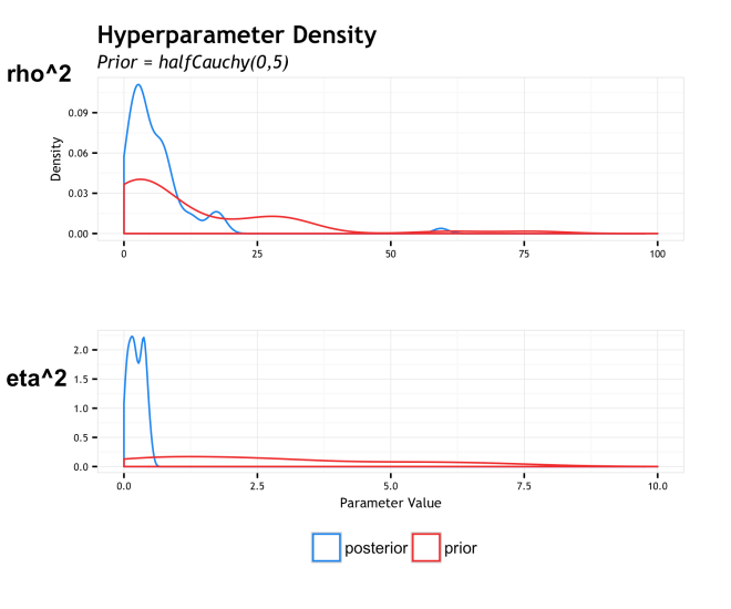
The distribution of these parameters is visualized in the plot below. Note that this is only a single chain simulation with 150 iterations; that will no do for your real world models. However, for getting code off the ground with made up data, it demonstrates the concept. From here, there are many ways to go. Depending on your problem, the length scale might have a very significant meaning and you can do inference on the posterior of that variable. Perhaps you will find that the estimations are way off from what you expect and the you further explore your data. Maybe you find out it is best to fix it because the MAP is right were anticipated and you don’t want to spend CPU cycles on it. Those basic questions are the real crux of modeling and well beyond the scope of this code oriented post.

I hope some of the information here is educational, has some relevance, and is not too riddled with error. I find GPs a really interesting framework for prediction and inference. I have only scratched the surface and will continue to work at them and find applications in my archaeological area of interest. However, these are universal machines and can applied to pretty much any domain. I plan to post again about variations in the kernel and the affects of kernel manipulation, but I will save that for another time.

Any errors in this post are my own dumb fault and will be corrected; please contact me if you see anything. The code for all of these graphics and models is here.

notes:

The R code for all analysis and plots can be found in a gist here, as well as the three Stan model codes, here gp-sim_SE.stan, gp-predict_SE.stan,and GP_estimate_eta_rho_SE.stan

> sessionInfo()
 R version 3.2.2 (2015-08-14)
 Platform: x86_64-apple-darwin13.4.0 (64-bit)
 Running under: OS X 10.10.5 (Yosemite)

locale:
 [1] en_US.UTF-8/en_US.UTF-8/en_US.UTF-8/C/en_US.UTF-8/en_US.UTF-8

attached base packages:
 [1] stats graphics grDevices utils datasets methods
 [7] base

other attached packages:
 [1] ggalt_0.3.0.9000 lattice_0.20-33 MASS_7.3-43
 [4] viridis_0.3.4 cowplot_0.6.2 matrixcalc_1.0-3
 [7] reshape2_1.4.1 plyr_1.8.3 rstan_2.9.0
 [10] ggplot2_2.1.0

loaded via a namespace (and not attached):
 [1] Rcpp_0.12.4 RColorBrewer_1.1-2 base64enc_0.1-3
 [4] tools_3.2.2 extrafont_0.17 digest_0.6.9
 [7] jsonlite_0.9.19 gtable_0.2.0 DBI_0.3.1
 [10] parallel_3.2.2 gridExtra_2.2.1 Rttf2pt1_1.3.3
 [13] httr_1.1.0 dplyr_0.4.3 stringr_1.0.0
 [16] htmlwidgets_0.6 maps_3.1.0 stats4_3.2.2
 [19] grid_3.2.2 inline_0.3.14 R6_2.1.2
 [22] plotly_3.4.13 tidyr_0.4.1 extrafontdb_1.0
 [25] magrittr_1.5 htmltools_0.3.5 scales_0.4.0
 [28] codetools_0.2-14 rsconnect_0.4.1.4 assertthat_0.1
 [31] proj4_1.0-8 colorspace_1.2-6 labeling_0.3
 [34] KernSmooth_2.23-15 ash_1.0-15 stringi_1.0-1
 [37] lazyeval_0.1.10 munsell_0.4.3

2 thoughts on “Gaussian Process Hyperparameter Estimation”

Tim Mastny says:

Hey thanks for the great blog post. I’ve noticed that your James Keirstead link is broken. Do you know if the website has moved, or if the post is archived elsewhere?

Thanks

LikeLike

November 13, 2017 at 7:55 pm Reply
1. Mdharris says:
  
  Hello Tim, good catch! There is a bit of his work mirrored on R-bloggers: https://www.r-bloggers.com/gaussian-process-regression-with-r/
  and this gist: https://gist.github.com/jkeirstead/2312411
  Also check out Michael Betancourt’s 3 part series on GP: https://betanalpha.github.io/assets/case_studies/gp_part1/part1.html
  Thanks for reading!
  
  LikeLike
  
  November 13, 2017 at 8:02 pm Reply

Quantitative Archaeology

thoughts, models, and ephemera

Gaussian Process Hyperparameter Estimation

code:

The Squared Exponential Kernel

To Fix or to Estimate?

The SE Kernel Prior

The Gaussian Process

How the prior effects our model

GP Kernel Hyperparameter Estimation

notes:

2 thoughts on “Gaussian Process Hyperparameter Estimation”

Leave a Reply Cancel reply

code:

The Squared Exponential Kernel

To Fix or to Estimate?

The SE Kernel Prior

The Gaussian Process

How the prior effects our model

GP Kernel Hyperparameter Estimation

notes:

Share this:

Like this:

Related

2 thoughts on “Gaussian Process Hyperparameter Estimation”

Leave a Reply Cancel reply