The alluvial plot and Sankey diagram are both forms of the more general Flow diagrams. These plot types are designed to show the change in magnitude of some quantity as it flows between states. The states (often on the x-axis) can be over space, time, or any other discreet index. While the alluvial and Sankey diagrams are differentiated by the way that the magnitude of flow is represented, they share a lot in common and are often used interchangeably as terms for this type of plot. The packages discussed here typically invoke (correctly IMHO) the term “alluvial”, but be aware that Sankey will also come up in discussion of the same plot format. Also, check out @timelyportfolio’s new post on interactive JS Sankey-like plots.

Motivation
This post is motivated by a few recent events; 1) I required a visualization of the “flow” of decisions between two models; 2) my tweet asking for ways to achieve this in R; 3) the ensuing discussion within that thread; and 4) a connected thread on Github covering some of the same ground. I figured I would put this post together to address two issues that arose in the events above:
- A very basic introduction into the landscape of non-JS/static alluvial plot packages in R.
- Within these packages, if it is possible to use ordered factors to reorder the Y axis to change the order of strata.
To those ends, below is a surficial and brief look at how to get something out of each of these packages and approaches to reordering. These packages have variable levels of documentation, but say to say that for each one you can learn a lot more than you can here. However, it is a corner of data vis in R that is not as well known as some others. This view is justified by the twitter and Github threads on the matter. Of course as these packages develop, this code may fall into disrepair and new options will be added.
R packages used in this post
library("dplyr")
library("ggplot2")
library("alluvial")
# devtools::install_github('thomasp85/ggforce')
library("ggforce")
# devtools::install_github("corybrunson/ggalluvial")
library("ggalluvial")
library("ggparallel")
Global parameters
To make life a little easier, I put a few common parameters up here. If you plan to cut-n-paste code from the plot examples, note that you will need these values as well to make them work as-is.
Part of the issue in this post is to look at what ordering factors does to change (or more likely not change) the vertical order of strata. Here I set factor levels to “A”, “C”, “B” and will use this in the examples below to see what using factors does to each plotting function. This order was used because it does not follow either ascending or descending alphabetical order.
A_col <- "darkorchid1"
B_col <- "darkorange1"
C_col <- "skyblue1"
alpha <- 0.7 # transparency value
fct_levels <- c("A","C","B")
Simulate data for plotting
The initial thread I started on Twitter was in response to my need to visualize the “flow” of decisions between two models. One model is the results of a predictive model I made a few years back; these values are labelled as “Modeled” in the data below. The other model is a implementation of the statistical model where individual decisions were made to change predictions or leave them the same; here the implementation is labelled “Tested”. The predictions that were decided upon are simply called “A”, “B”, and “C” here, but these could be any exhaustive set of non-overlapping values. Other examples could be “Buy”, “Sell”, and “Hold” or the like. The point of the graphic is to visually represent the mass and flow of values between the statistical model and the implemented model. Sure this can be done is a table (as the one down below), but it also lends to a visual approach. Is it the best way to visualize these data? I have no idea, but it is the one that I like.
The dat_raw is the full universe of decisions shared by the two models (all the data). The dat data frame is the full data aggregated by decision pairs with the addition of a count of observations per pair. You will see in the code for the plots below, each package ingests the data in a slightly different manner. As such, dat and dat_raw serve as the base data for the rest of the post.
dat_raw <- data.frame(Tested  = sample(c("A","B","C"),100,
                                  replace = TRUE,prob=c(0.2,0.6,0.25)),
                  Modeled = sample(c("A","B","C"),100,
                                  replace = TRUE,prob=c(0.56,0.22,0.85)),
                  stringsAsFactors = FALSE)
dat <- dat_raw %>%
  group_by(Tested,Modeled) %>%
  summarise(freq = n()) %>%
  ungroup()
| Tested | Modeled | freq |
|---|---|---|
| A | A | 7 |
| A | B | 3 |
| A | C | 8 |
| B | A | 25 |
| B | B | 7 |
| B | C | 27 |
| C | A | 8 |
| C | B | 4 |
| C | C | 11 |
ggforce
ggforce (https://github.com/thomasp85/ggforce)
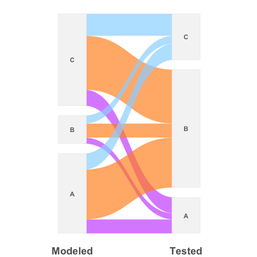
ggforce is Thomas Lin Pedersen’s package for adding a range of new geoms and functionality to ggplot2. The geom_parallel_sets used to make the alluvial chart here is only available in the development version installed from Github. ggforce provides a helper function gather_set_data() to get the dat in the correct format for ggplot; see below.
Ordering – By default ggforce orders the strats (i.e. “A”, “B”, “C”) based on alphabetical order from the bottom up. There is no obvious way to change this default, but I am looking into it.
dat_ggforce <- dat  %>%
  gather_set_data(1:2) %>%        # <- ggforce helper function
  arrange(x,Tested,desc(Modeled))

ggplot(dat_ggforce, aes(x = x, id = id, split = y, value = freq)) +
  geom_parallel_sets(aes(fill = Tested), alpha = alpha, axis.width = 0.2,
                     n=100, strength = 0.5) +
  geom_parallel_sets_axes(axis.width = 0.25, fill = "gray95",
                          color = "gray80", size = 0.15) +
  geom_parallel_sets_labels(colour = 'gray35', size = 4.5, angle = 0, fontface="bold") +
  scale_fill_manual(values  = c(A_col, B_col, C_col)) +
  scale_color_manual(values = c(A_col, B_col, C_col)) +
  theme_minimal() +
  theme(
    legend.position = "none",
    panel.grid.major = element_blank(),
    panel.grid.minor = element_blank(),
    axis.text.y = element_blank(),
    axis.text.x = element_text(size = 20, face = "bold"),
    axis.title.x  = element_blank()
    )
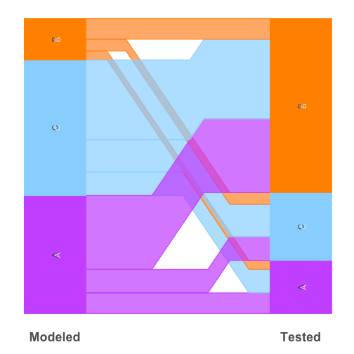
ggforce with factors
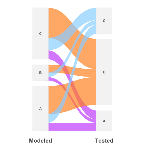
Attempting to use factor levels for ggforce has an interesting effect. Here you can see that while the strata are still ordered as the default alphabetical order, the bands that flow between them are reordered according to factors.
To my knowledge there is no direct way to reorder strata in ggforce. With a brief review of the ggforce code, I think the ordering is established in this line data$split <- as.factor(data$split), but not 100% sure. More work to be done here…
dat_ggforce2 <- dat_ggforce %>%
  mutate_at(vars(Modeled, Tested),
            funs(factor(., levels = fct_levels)))

ggplot(dat_ggforce2, aes(x = x, id = id, split = y, value = freq)) +
  geom_parallel_sets(aes(fill = Tested), alpha = alpha, axis.width = 0.2,
                     n=100, strength = 0.5) +
  geom_parallel_sets_axes(axis.width = 0.25, fill = "gray95",
                          color = "gray80", size = 0.15) +
  geom_parallel_sets_labels(colour = 'gray35', size = 4.5, angle = 0, fontface="bold") +
  scale_fill_manual(values  = c(A_col, C_col, B_col)) +
  scale_color_manual(values = c(A_col, C_col, B_col)) +
  theme_minimal() +
  theme(
    legend.position = "none",
    panel.grid.major = element_blank(),
    panel.grid.minor = element_blank(),
    axis.text.y = element_blank(),
    axis.text.x = element_text(size = 20, face = "bold"),
    axis.title.x  = element_blank()
  )
ggalluvial
ggalluvial (https://github.com/corybrunson/ggalluvial)
ggalluvial is similar to ggforce in that it uses a custom geom to integrate into ggplot2; a good approach. A pro of this package is that the data does not need a special helper function to get it prepared for plotting. This package takes the basic aggregated counts of dat. Note that the default strata ordering is alphabetical from the top down.
dat_ggalluvial <- dat

ggplot(dat_ggalluvial,
       aes(weight = freq, axis1 = Modeled, axis2 = Tested)) +
  geom_alluvium(aes(fill = Tested, color = Tested),
                width = 1/12, alpha = alpha, knot.pos = 0.4) +
  geom_stratum(width = 1/6,color = "grey") +
  scale_fill_manual(values  = c(A_col, B_col, C_col)) +
  scale_color_manual(values = c(A_col, B_col, C_col)) +
  geom_text(stat = "stratum", label.strata = TRUE) +
  scale_x_continuous(breaks = 1:2, labels = c("Modeled", "Tested")) +
  theme_minimal() +
  theme(
    legend.position = "none",
    panel.grid.major = element_blank(),
    panel.grid.minor = element_blank(),
    axis.text.y = element_blank(),
    axis.text.x = element_text(size = 18, face = "bold")
  )

ggalluvial with factors
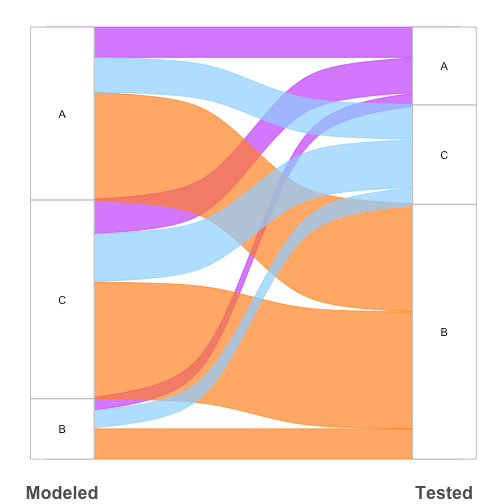
Another pro of this package is that is recognizes the factor levels in reordering the strata. In the plot below, notice the arrangement of “A”, “C”, and “B”. This can be very helpful when strata order matters, as is my use case.
dat_ggalluvial2 <- dat_ggalluvial %>%
  mutate_at(vars(Modeled, Tested),
            funs(factor(., levels = fct_levels)))

ggplot(dat_ggalluvial2,
       aes(weight = freq, axis1 = Modeled, axis2 = Tested)) +
  geom_alluvium(aes(fill = Tested, color = Tested),
                width = 1/12, alpha = alpha, knot.pos = 0.4) +
  geom_stratum(width = 1/6,color = "grey") +
  scale_fill_manual(values  = c(A_col, C_col, B_col)) +
  scale_color_manual(values = c(A_col, C_col, B_col)) +
  geom_text(stat = "stratum", label.strata = TRUE) +
  scale_x_continuous(breaks = 1:2, labels = c("Modeled", "Tested")) +
  theme_minimal() +
  theme(
    legend.position = "none",
    panel.grid.major = element_blank(),
    panel.grid.minor = element_blank(),
    axis.text.y = element_blank(),
    axis.text.x = element_text(size = 18, face = "bold")
  )
alluvial
alluvial (https://cran.r-project.org/web/packages/alluvial/vignettes/alluvial.html)
The alluvial package takes a different approach than those above as it is not based on ggplot2, but instead on base R plotting. The look is similar to proceeding packages, but it cannot be extended with additional calls to ggplot2 options as in the above plots. Note that the colors of each strata are assigned to the left hand site (e.g. as Modeled “C” is all blue), as opposed to the above packages where the color of the strata is based on the right hand side.
dat_alluvial <- dat %>%
  dplyr::select(Modeled, Tested, freq)

alluvial::alluvial(dat_alluvial[,1:2], freq=dat_alluvial$freq,
          xw=0.2, alpha=alpha,gap.width=0.1,
          col= c(A_col, B_col, C_col),
          border=c(A_col, B_col, C_col),
          blocks=TRUE, cex = 1.1, cex.axis = 1.5
          )

alluvial with factors
The alluvial package also responds to factor levels, but in the reverse order as compared to ggalluvial with “A” at the bottom. As above, the color is associated with the strata label on the left hand side.
dat_alluvial2 <- dat_alluvial %>%
  mutate_at(vars(Modeled, Tested),
            funs(factor(., levels = fct_levels)))

alluvial::alluvial(dat_alluvial2[,1:2], freq=dat_alluvial$freq,
          xw=0.2, alpha=alpha,gap.width=0.1,
          col= c(A_col, B_col, C_col),
          border=c(A_col, B_col, C_col),
          blocks=TRUE, cex = 1.1, cex.axis = 1.5
          )

ggparallel
ggparallel (https://github.com/heike/ggparallel)
Finally, ggparallel takes a somewhat different approach to visualizing strata. Instead of using splines to fluidly connect each side, this package uses angular bands; it is an interesting look! As sort of a hybrid between the approaches above, this package uses ggplot2 as a base, but wraps it in an overarching function ggparallel() instead of a custom geom. This may have some effects on flexibility, but it is overall an easy to use package. Default ordering is alphabetical order from the bottom up.
Note that the package does have options for the parameter order. values of -1, 0, and 1 are available for ordering by decreasing alphabetical/numerical order, increasing alphabetical/numerical order, or by the order presented in the data (default). This can be used to a variety of effects. However, below the
# @param order flag variable with three levels -1, 0, 1 for levels in
#    decreasing order, levels in increasing order and levels unchanged. This
#    variable can be either a scalar or a vector

ggparallel(list("Modeled", "Tested"), data = dat_raw,
           alpha = alpha, order = 0) +
  scale_fill_manual(values  = c(A_col, B_col, C_col, A_col, B_col, C_col)) +
  scale_color_manual(values  = c(A_col, B_col, C_col, A_col, B_col, C_col)) +
  theme_minimal() +
  theme(
    legend.position = "none",
    panel.grid.major = element_blank(),
    panel.grid.minor = element_blank(),
    axis.text.y = element_blank(),
    axis.title.y = element_blank(),
    axis.text.x = element_text(size = 18, face = "bold")
  )
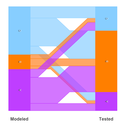
ggparallel with factors
Here the factor levels can be used to assign the order of the strata and the order parameter can be used to sort them increasing or decreasing. This is more flexible that other packages, but you have to like the distinct look in order to run with it.
# @param order flag variable with three levels -1, 0, 1 for levels in
#    decreasing order, levels in increasing order and levels unchanged. This
#    variable can be either a scalar or a vector

dat_raw2 <- dat_raw %>%
  mutate_at(vars(Modeled, Tested),
            funs(factor(., levels = fct_levels)))

ggparallel(list("Modeled", "Tested"), data = dat_raw2,
           alpha = alpha, order = 0) +
  scale_fill_manual(values  = c(A_col, B_col, C_col, A_col, B_col, C_col)) +
  scale_color_manual(values  = c(A_col, B_col, C_col, A_col, B_col, C_col)) +
  theme_minimal() +
  theme(
    legend.position = "none",
    panel.grid.major = element_blank(),
    panel.grid.minor = element_blank(),
    axis.text.y = element_blank(),
    axis.title.y = element_blank(),
    axis.text.x = element_text(size = 18, face = "bold")
  )
##Notes:
1) This post is created using the knit2wp() function in the wonderful RWordPress package along with knitr
sessionInfo()
## R version 3.4.0 (2017-04-21)
## Platform: x86_64-apple-darwin15.6.0 (64-bit)
## Running under: macOS Sierra 10.12.5
##
## Matrix products: default
## BLAS: /System/Library/Frameworks/Accelerate.framework/Versions/A/Frameworks/vecLib.framework/Versions/A/libBLAS.dylib
## LAPACK: /Library/Frameworks/R.framework/Versions/3.4/Resources/lib/libRlapack.dylib
##
## locale:
## [1] en_US.UTF-8/en_US.UTF-8/en_US.UTF-8/C/en_US.UTF-8/en_US.UTF-8
##
## attached base packages:
## [1] stats     graphics  grDevices utils     datasets  methods   base
##
## other attached packages:
##  [1] alluvial_0.1-2     Gmisc_1.5          htmlTable_1.9      Rcpp_0.12.13       ggparallel_0.2.0
##  [6] ggalluvial_0.3     ggforce_0.1.1      RWordPress_0.2-3   devtools_1.13.3    knitr_1.17
## [11] extrafont_0.17     stringr_1.2.0      bindrcpp_0.2       dplyr_0.7.4        purrr_0.2.3
## [16] readr_1.1.1        tidyr_0.7.1        tibble_1.3.4       ggplot2_2.2.1.9000 tidyverse_1.1.1
## [21] raster_2.5-8       sp_1.2-5
##
## loaded via a namespace (and not attached):
##  [1] nlme_3.1-131        bitops_1.0-6        lubridate_1.6.0     RColorBrewer_1.1-2  httr_1.3.1
##  [6] rprojroot_1.2       tools_3.4.0         backports_1.1.0     rgdal_1.2-8         R6_2.2.2
## [11] rpart_4.1-11        Hmisc_4.0-3         lazyeval_0.2.0      colorspace_1.3-2    nnet_7.3-12
## [16] withr_2.0.0         gridExtra_2.2.1     tidyselect_0.2.0    mnormt_1.5-5        curl_3.0
## [21] compiler_3.4.0      git2r_0.19.0        extrafontdb_1.0     rvest_0.3.2         xml2_1.1.1
## [26] labeling_0.3        scales_0.5.0.9000   checkmate_1.8.4     psych_1.7.5         digest_0.6.12
## [31] foreign_0.8-67      rmarkdown_1.6       base64enc_0.1-3     pkgconfig_2.0.1     htmltools_0.3.6
## [36] highr_0.6           htmlwidgets_0.9     rlang_0.1.2         readxl_1.0.0        XMLRPC_0.3-0
## [41] bindr_0.1           jsonlite_1.5        acepack_1.4.1       RCurl_1.95-4.8      magrittr_1.5
## [46] kableExtra_0.5.2    Formula_1.2-2       Matrix_1.2-9        munsell_0.4.3       abind_1.4-5
## [51] stringi_1.1.5       yaml_2.1.14         MASS_7.3-47         plyr_1.8.4          grid_3.4.0
## [56] parallel_3.4.0      forcats_0.2.0       udunits2_0.13       deldir_0.1-14       lattice_0.20-35
## [61] splines_3.4.0       haven_1.0.0         hms_0.3             markdown_0.8        reshape2_1.4.2
## [66] XML_3.98-1.9        glue_1.1.1          evaluate_0.10.1     latticeExtra_0.6-28 data.table_1.10.4
## [71] modelr_0.1.0        tweenr_0.1.5        Rttf2pt1_1.3.4      cellranger_1.1.0    gtable_0.2.0
## [76] polyclip_1.6-1      assertthat_0.2.0    mime_0.5            broom_0.4.2         survival_2.41-3
## [81] forestplot_1.7.2    memoise_1.1.0       cluster_2.0.6       units_0.4-6         concaveman_1.0.0

Great post but packages referenced have been updated and a lot of the functions leveraged like `gather_set_data` have been removed from ggforce 😦
LikeLike