Quick Way longer then expected post and some code for looking into the estimation of kernel hyperparameters using STAN HMC/MCMC and R.  I wanted to drop this work here for safe keeping. Partially for the exercise of thinking it through and writing it down, but also because it my be useful to someone.  I wrote a little about GP in a previous post, but my understanding is rather pedestrian, so these explorations help.  In general GPs are non-linear regression machines that utilize a kernel to reproject your data into a larger dimensional space in order to represent and better approximate the function we are targeting.  Then using a covariance matrix calculated from that kernel, a multivariate Gaussian posterior is derived.  The posterior can then be used for all of the great things that Bayesian analysis can do with a posterior.

Read lots more about GP here…. Big thanks to James Keirstead for blogging a bunch of the code that I used under the hood here and thanks to Bob Carpenter (github code) and the Stan team for great software with top-notch documentation.

code:

The R code for all analysis and plots can be found in a gist here, as well as the three Stan model codes, here gp-sim_SE.stan, gp-predict_SE.stan,and GP_estimate_eta_rho_SE.stan

 

The hyperparameters of topic here are parameters of the kernel within the GP algorithm.  As with other algorithms that use kernels, a number of functions can be used based on the type of generative function you are approximating.  The most commonly used kernel function for GP (and seemingly Support Vector Machines) is the Squared Exponential (SE), also known as the Radial Basis Function (RBF), Gaussian, or Exponentiated Quadratic function.

The Squared Exponential Kernel

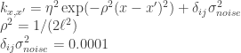
The SE kernel is a negative length scale factor rho () times the square distance between data points () all multiplied by a scale factor eta ().  Rho is a shorthand for the length scale which is often written as a denominator as shown below. Eta is a scale factor that determines how far the function varies from the mean. Finally sigma squared () at the end is the value for the diagonal elements of the matrix where (). This last term is not necessarily part of the kernel, but is instead a jitter term to set zero to near zero for numeric reasons.  The matrix created by this function is positive semi-definite and composed of the distance between observations scaled by rho and eta. Many other kernels (linear, periodic, linear * periodic, etc…) can be used here; see the kernel cookbook for examples.

To Fix or to Estimate?

In this post, models are created where  , , and  are all fixed, as well as a model where   is fixed and  and  are free.  In the MCMC probabilistic framework, we can fix  and  or any parameter for the most part, or estimate them. To this point, there was a very informative and interesting discussion on stan-users mailing list about why you might want to estimate the SE kernel hyperparameters.  The discussion generally broke across the lines of A) you don’t need to estimate these, just use relatively informative priors based on your domain knowledge, and B) of course you want to estimate these because you may be missing a large chunk of function space and uncertainty if you do not. The conclusion to the thread is a hedge to try it both ways, but there are great bits of info it there regardless.

So while the greatest minds in Hamiltonian Monte Carlo chat about it, I am going to just naively work on the Stan code to do these estimations and see where it takes me.  Even if fixed with informative priors is the way to go, I at least want to know how to write/execute the model that estimates them. So here we go.

Continue reading “Gaussian Process Hyperparameter Estimation” →