Reproducible research… so hot right now. This post is about a way to use “Containers” to conduct analysis in a more reproducible way. If you are familiar with Docker containers and reproducibility, you can probably skip most of this and check out the liftr code snippets towards the end. If you are like, “what the heck is this container business?”, then I hope that this post gives you a bit of insight on how to turn basic R scripts and Rmarkdown into fully reproducible computing environments that anyone can run. The process is based on the Docker container platform and the liftr R package. So if you want to hear more about using liftr for reproducible analysis in R, please continue!

• Concept – Learn to create and share a Dockerfile with your code and data to more faithfully and accurately reproduce analysis.
• User Level – Beginner to intermediate level R user; some knowledge of Rmarkdown and the concept of reproducibility
• Requirements – Recent versions of R and RStudio; Docker; Internet connection
• Tricky Parts
  • Installing Docker on your computer (was only 3 clicks to install on my Mac Book)
  • Documenting software setup in YAML-like metadata (A few extra lines of code)
  • Conceptualizing containers and how they fit with a traditional analysis workflow (more on that below)
• Pay Off
  • A level-up in your ability to reproduce your own and others code and analysis
  • Better control over what your software and analysis is doing
  • Confidence that your analytic results are not due to some bug in your computer/software setup

More than just sharing code…

So you do your analysis in R (that is awesome!) and you think reproducibility is cool. You share code, collaborate, and maybe use Git Hub occasionally, but the phrase ‘containerization of computational environments’ doesn’t really resonate. Have no fear, you are not alone! Sharing your code and data is a great way to take advantage of the benefits of reproducible research and well documented in a variety of sources. Marwick 2016 and Marwick and Jacobs 2017 as leading examples. However, limiting ourselves to thinking of reproducibility as only involving code and data ignores the third and equally crucial component; the environment.

Simply, the environment of the analysis includes the computer’s software, settings, and configuration on which it was run. For example, if I run an analysis on my Mac with OSX version something, and Rstudio version 1.1.383, a few packages, and program XYZ installed it may work perfectly in that computational environment. If I then share the code with a co-worker and they try to run it on a computer with Windows 10, Rstudio 0.99b, and clang4, but not rstan and liblvm203a the code will fail with a variety of hard to decipher error messages. The process is decidedly not reproducible. Code and data are in place, but the changes to the computational environment thwart attempts are reproducing the analysis.

At this point, it may be tempting to step back and claim that it is user #2’s prerogative to make an environment that will run the code; especially if you won’t have to help them fix this issue. However, we can address this problem in straightforward way, uphold the ethos of reproducibility, and make life less miserable for our future selves. This is where Docker and containers come into play.

So what is a container?

Broadly speaking, a container is a way to put the software & system details of on one computer into a set of instructions that can be recreated on another computer; without changing the second computers underlying software & system. This is the same broad concept of Virtual machines, virtual environments, and containerization. Simply, I can make your computer run just like my computer. This magic is achieved by running the Docker platform on your computer and using a Dockerfile to record the instructions for building a specific computational environment.

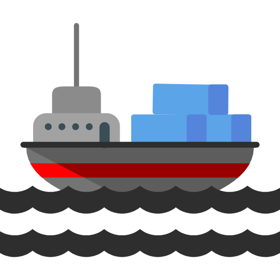
There is a ton about this that can be super complex and float well-above ones head. Fortunately, we don’t need to know all the details to use this technology! The name “container” is a pretty straight ahead metaphor for what this technology does. Specifically a shipping container is a metal box of a standard size that stacks up on any ship and moves to any port regardless of what it carries and what language is spoken. It is a standardized unit of commerce. In that sense, the Docker container is a standardized shipping box for a computer environment that fits in a single file, ships to any computer, and contains any odd assortment of software provided it is specified in the Dockerfile. To this end, the idea is that you can pack the relevant specifics of your computer, software, versions, packages, etc… into a container and ship it with your code and data allowing an end user to recreate your computing environment and run the analysis. Reproducibility at its finest!

 

The container metaphor is good and it fits well with software engineers shipping applications here and there. From the analysis point of view, a more applicable metaphor may be that of a bubble. A container is a metaphor of commerce, a bubble is a metaphor of boundaries; what happens in the bubble stays in the bubble. Docker allows you to both put your analysis and run someones else analysis in a bubble. The air inside the bubble (the environment) is composed of a list of ingredients specified in the Dockerfile. Code that runs in the bubble environment do not affect your system outside of the bubble. This is the beauty of the reproducible environment approach; bubbles/containers isolate the code, data, and analysis and unify the reproducibility triumvirate. Best yet, creating the computational environment containers is not as difficult as it sounds. This post shows you how to use the liftr package in R to take any analysis and make it into a reproducible package of code, data, and an environment.

Analysis in a bubble

I made some graphics to try to visualize the bubble metaphor as an abstract workflow. We will fill in details later. Referring to the graphic below, the process starts at (1) with your analysis in a Rmarkdown document and your data stored locally. If you are not families with formatting an analysis in Rmarkdown, consult this brief tutorial, this arXiv PDF, or this Rstudio Community post. Once your analysis in complete, or nearly so, you proceed to (2) where the Rmarkdown is wrapped in a bubble and executed in its entirety. The really important part here is that when the analysis is run in the bubble, it is run with only the software and configuration that you put into the bubble, not the software and configuration you created the analysis in at step (1). Noting that you can complete step (1) within a step (2) bubble if you are comfortable with that. When the analysis is run in (2) any dependency on your local environment that is not specifically placed in the bubble environment will become clear as the code errors and likely fails. Through these failures you will recognize additional things that you need to put in the bubble to make the analysis run without failure. These are very likely the bits and pieces that would cause the code to fail if a co-worker tried to run the Rmarkdown on their own machine without the protective bubble.

Once the bubble is properly specified and the code runs successfully in (2) you end up with two primary outputs; (3) the reproducible research compendium containing your data, code, and the specification of the bubble environment (the Dockerfile), and (4) the PDF, HTML, or MS Word output of the analysis. With the compendium from (3) and output from (4) you have all parts of a full and reproducible analysis. From here, it is easy to post such a compendium to Git Hub or similar cloud-based platform (5) for version control, collaboration, archiving, and distribution.

The workflow depicted above is how your compendium can be used to foster new works or be run in its original form to reproduce your results. Once your compendium is cloned (6), the instructions to rebuild the computational environment are used to re-create the analysis bubble on a new computer (7) and the Rmarkdown is executed. If this is done with the original data, it would result in a reproduced output (9) from original analysis. Otherwise, if new data are utilized or the analysis is altered, it would result in a new compendium (8) that can therefore be shared (10) and output (11). Each time the bubble is created from the recipe from the first analysis, the computation environment is reproduced agnostic of the underlying software & hardware.

The justification for using the light-hearted and non-technical analogy of a bubble to represent the complexities of containerization is that for the users that this workflow would benefit most, it is best to abstract away as much of the details of Docker and provide a system that works with low friction. The busy scientist that is spending too much time troubleshooting cross-system collaboration can benefit hugely from this technology. However, they can only take advantage of it is the barrier to entry is low enough to justify taking time away from research to learn a new technique. This is very problem that the liftr package is very effective at solving. Below, we will put the bubble metaphor into practice using the liftr package approach. If you want to follow up with a more in depth read into containers and reproducibility check out the Ropensci Docker Tutorial

Setting the stage for reproducible analysis

There are any number of use cases where we may want to share a reproducible script. A very simple and general example is the review/discussion of an analysis with collaborating colleagues. A lot of time and understanding can be lost when sharing a jpeg of a plot and an excel file of coefficients. More ideally, you can share the full analysis so that collaborators can better understand the approach, run the results, and tweak as needed. I made an example .Rmd for such an analysis (download here if you want to try the examples below). The exploration of liftr below will utilized this example.

Creating a Reproducible Analysis with the Liftr Package

Created by Nan Xiao (Twitter), the liftr package:

aims to solve the problem of persistent reproducible reporting. To achieve this goal, it extends the R Markdown metadata format, and uses Docker to containerize and render R Markdown documents.

The magic and beauty of liftr is that it greatly simplifies the process of dealing with the Docker container (aka the Bubble). Without liftr, you would have to do something like writing a configuration file from scratch, spinning-up the container, running the script, and shutting it down afterwards. While to some that is not a difficult task, to a newcomer to this approach that is fairly intimidating. With liftr you simply add a few lines of metadata to the Rmd header to specify your packages and run a few functions on that Rmd file to configure, build, and purge the container. The entire process of dealing with Docker is abstracted away and executable all from Rstudio. It does the heavy lifting… (pun intended) Best yet, the Dockerfile built in the process can then follow with your Rmd and data as a compendium to allow others to render your analysis in a container on their system. To see how this fits into the schematic developed above:

Adding some details to the bubble metaphor, step (1) is the local Rmarkdown .Rmd file that has the extra liftr specific metadata in the YAML header (example in the section below). Step (2) is to execute liftr::lift() on the Rmd file, thereby creating the makeup of the bubble/container in the way of a Dockerfile. Step (3) combines the Rmd and the Dockerfile in liftr::render_docker() to build the bubble (4) within which the code is executed. The outputs of (4) include the rendered Rmd in the form of PDF, HTML, or MS Word doc as (5) and a new Docker YAML file (6) that hold specifics of the container created in (4). This file can then be used by lifr::purge_image() and liftr::purge_container() functions to clean up your computer and get rid of the bubble. The final level of detail for this process is described below in a step-by-step use case of liftr on the Rmd available to download above.

The illustration below from the liftr website describes the same general process:

Putting liftr to work

liftr is incredibly easy to use for many use cases. It can also be extended in a few ways for not-so-basic use cases, but the basic case will cover a lot of ground. The basic steps here are:

1. Add liftr metadata to Rmd header
2. Use the liftr::lift() function on the Rmd file to create the Dockerfile
3. Use the liftr::render_docker() function on the same Rmd file resulting in:
   • building the Docker container and executing your analysis code from the Rmd
   • rendering the desired output; PDF, HTML, Word doc.
   • creating a Docker YAML file (liftr_analysis_rbg.docker.yml) that leaves instructions for liftr to remove the container and Docker images.
4. Use the liftr::purge_image() and/or liftr::purge_container() functions to clean up!

Step 1 – Rmd header metadata

Using the example liftr_analysis_rbg.Rmd I created and linked to above, the syntax for the header metadata is quite simple – see below. Under the typical Rmd header information, if a section initiated with liftr:. This these liftr vignette covers the various options you can use in this header; I use a pretty minimal setup here. The from: tag is where you choose the Docker image that serves as the base of our environment. These images are selected from the Rocker library of images. This is basically a prepackaged version of R and all the stuff that is needed to run it. There are some options rich images such as tidyverse, but take not of the file sizes before you select one for your need. In addition to the base image, you also modify your metadata to detail the packages that need to be installed to execute your Rmd. In this case, I used the CRAN packages tufte, tidyverse, archdata, and ggefects. Including the packages here tells Docker to install these on top of the r-base image before running the Rmd script. Similarly, if there are packages from Git hub or even non-R package software that needs installing, it can be specified here or in a separate file; see the liftr vignette for more details.

---
title: "Marginal Effects of Elements in RBGlass1 Data"
author: "Matthew Harris <<me@me.com>>"
date: "`r Sys.Date()`"
output:
  tufte::tufte_html: default
liftr:
  from: "rocker/r-base:latest"
  maintainer: "Matthew Harris"
  email: "me@me.com"
  cran:
    - tufte
    - tidyverse
    - archdata
    - ggeffects
---

Step 2, 3, and 4 – build, render, purge the container

I seriously wish there was more to it than this; I have stretched out this blog post to a pinnacle of five lines of code! For better or worse, that is just how simple liftr makes this process. Again, if you want to follow along with the example Rmd I created, feel free to download it and change the directory path below to that file.

The code below follows the steps outlined above. liftr::lift(Rmd) creates the Dockerfile and leaves it in the same directory as the Rmd. Then liftr::render_docker(Rmd) builds the Docker container based on the Dockerfile; grab a tea/coffee/beverage-of-choice as this may take some time… The building of the container plays out live across your R console with lots of frightening red text and building stuff; keep your eye out for errors and omitted packages. After building, the container automatically executes the Rmd within that container environment. The output of the Rmd will end up in the same directory as the Rmd. Finally liftr::purge_image(...) removes the image you just made. From here, the directory you linked to will have the output of the Rmd as a PDF, HTML, or Word doc (as specified in the Rmd header) and the Dockerfile suitable for reusing on your system or another system with Docker installed.

dir_example = "/file/path/to/Rmd/"
input = paste0(dir_example, "liftr_analysis_rbg.Rmd")
liftr::lift(input)
liftr::render_docker(input)
liftr::purge_image(paste0(dir_example, "liftr_analysis_rbg.docker.yml"))

To get a sense of what the liftr::lift() function is doing, take a look at the Dockerfile (below) created by this function. In addition to importing the specified Rocker base image, the Dockerfile relays a series of instructions for building the container environment and installing the software & packages required for your analysis. As you may imagine, without liftr it would be mostly up to you to build this file and know what goes into it. Fortunately, this package takes away much of that burden (in addition to the amazing Rocker base images).

FROM rocker/r-base:latest

MAINTAINER Matthew Harris <me@me.com>

# System dependencies for required R packages
RUN  rm -f /var/lib/dpkg/available \
  && rm -rf  /var/cache/apt/* \
  && apt-get update -qq \
  && apt-get install -y --no-install-recommends \
    ca-certificates \
    libssl-dev \
    libcurl4-openssl-dev \
    libxml2-dev \
    git

# Pre-compiled pandoc required by rmarkdown
# Version from: https://github.com/metacran/r-builder/blob/master/pkg-build.sh
# Scripts from: https://github.com/jangorecki/dockerfiles/blob/master/r-pkg/Dockerfile
RUN PANDOC_VER="1.17.2" \
  && PANDOC_DIR="/opt/pandoc" \
  && PANDOC_URL="https://s3.amazonaws.com/rstudio-buildtools/pandoc-${PANDOC_VER}.zip" \
  && mkdir -p "${PANDOC_DIR}" \
  && wget --no-check-certificate -O /tmp/pandoc-${PANDOC_VER}.zip ${PANDOC_URL} \
  && unzip -j /tmp/pandoc-${PANDOC_VER}.zip "pandoc-${PANDOC_VER}/linux/debian/x86_64/pandoc" -d "${PANDOC_DIR}" \
  && chmod +x "${PANDOC_DIR}/pandoc" \
  && ln -s "${PANDOC_DIR}/pandoc" /usr/local/bin \
  && unzip -j /tmp/pandoc-${PANDOC_VER}.zip "pandoc-${PANDOC_VER}/linux/debian/x86_64/pandoc-citeproc" -d "${PANDOC_DIR}" \
  && chmod +x "${PANDOC_DIR}/pandoc-citeproc" \
  && ln -s "${PANDOC_DIR}/pandoc-citeproc" /usr/local/bin \
  && rm -f /tmp/pandoc-${PANDOC_VER}.zip

RUN Rscript -e "install.packages(c('devtools','knitr','rmarkdown','shiny','RCurl'), repos = 'https://cran.rstudio.com')"

RUN Rscript -e "source('https://cdn.rawgit.com/road2stat/liftrlib/aa132a2d/install_cran.R');install_cran(c('tufte','tidyverse','archdata','geffects'))"

RUN mkdir /liftrroot/
WORKDIR /liftrroot/

Notes:

• The container ship icon is modified from: https://www.shareicon.net/cargo-ship-shipping-and-delivery-shipping-navigation-transportation-boat-transport-808888