See executable Rstudio notebook of this post at this Github repo!
I have had a thing lately with aggregating analyses into sequences of purrr::map() function calls and dense tibbles. If I see a loop – map() it. Have many outputs – well then put it in a tibble. Better yet, apply a sequence of functions over multiple model outputs, put them in a tibble and map() it! That is the basic approach I take here for modeling over a sequence of random hyperparameters (Hypurrr-ameters???); plus using future to do it in parallel. The idea for the code in this post came after an unsettled night of dreaming in the combinatoric magnitude of repeated K-folds CV over the hyperparameters for a multilayer perceptron. anyway…

This post is based on the hyperparameter grid search example, but I am going to use it as a platform to go over some of the cool features of purrr that make it possible to put such an analysis in this tibble format. Further, I hope this post gives people some examples that make the idea of purrr “click”; I know it took me some time to get there. By no means a primer on purrr, the text will hopefully make some connections between the ideas of list-columns, purrr::map() functions, and purrr:nest() to show off what I interpret as the Tidy-Purrr philosophy. The part about using future to parallelize this routine is presented towards the end. If already know this stuff, then skip to the code examples at the end or see this repo. However, if you are purrr-curious, give it a read and check out some of the amazing tutorials out in the wild. If you want to interact with the code and this Rmd file, head over to this Github repo where you can launch an instance of Rstudio server and execute the code!
- Objective: Demonstrate an approach to randomly searching over model hyperparameters in parallel storing the results in a tibble.
- Pre-knowledge: Beginner to Moderate R; introductory modeling concepts; Tidy/Purrr framework
- Software:
R 3.4.0,tidyverse 1.2.1(containstibble,dplyr,purrr,tidyr, andggplot2),rsample 0.0.2,future 1.6.2

Optimizing hyperparameters
Hyperparameters are the tuning knobs for statistical/machine learning models. Basic models such as linear regression and GLM family models don’t typically have hyperparameters, but once you get into Ridge or Lasso regression and GAMs there are parts of the model that need tuning (e.g. penalties or smoothers). Methods such as Random Forest or Gradient Boosting, Neural Networks, and Gaussian Processes have even more tuning knobs and even less theory for how they should be set. Setting such hyperparameters can be a dark-art and require experience and a bit of faith. However, even with experience in these matters it is rarely clear what combination of hyperparameters will lead to the best out-of-sample prediction on a given dataset. For this reason, it is often desired to test over a range of hyperparameters to find the best pairing.
The major issue of searching hyperparameters is the computational cost of searching a wide range of values to avoid local minima, testing over a fine enough grid to avoid over-shooting minima, and estimating variance via bootstrapping or K-folds CV. For example, a model with two hyperparameters tested over K = 10 folds CV for the values of each hyperparameter equates to 10 x 10 x 10 = 1,000 models! A third hyperparameter is another order of magnitude. Needless to say, this adds up fast. While a handful or algorithms and approaches have been developed to deal with this, the most common method is a basic grid-search or a random search across a sequence of hyperparameters. In this example, I employ a random search, but changing it to grid-search is simple.
![]()
Purrr::map() and tibble
To preform hyperparameter search in a table, we can use the power of purrr to do the heavy lifting and the tibble to store the results/computations. The tibble is much like the basic data.frame in many respects, but differing in some key ways that allow for the purrr idiom to really flourish. One of those differences is that the tibble is very accommodating to dealing with all sorts of data stuffed into the grid cells. Often referred to a list-column, this behavior allows the each cell in a column to store lists, which themselves can contain any R data structure like lists, data,frames, tibbles, data, functions, etc… The toy example below shows how typical numeric and character data are stored in Col_A and Col_B while Col_C is a list with three elements, one for each row, containing the character vector "X","Y","Z". Finally, Col_D is a list that contains three elements (rows), each of which is also a list and contains three elements that are the XYZ character vector. Recursion!
library("tidyverse")
list_col_example <- tibble(Col_A = c(1,2,3),
                           Col_B = c("A","B","C"),
                           Col_C = list(c("X","Y","Z")),
                           Col_D = list(Col_C))
print(list_col_example)
## # A tibble: 3 x 4
##   Col_A Col_B     Col_C      Col_D
##   <dbl> <chr>    					<list>     					<list>
## 1     1     A <chr [3]> 					<list [3]>
## 2     2     B <chr [3]> 					<list [3]>
## 3     3     C <chr [3]> 					<list [3]>
This recursive storage is really powerful! In this example, we take advantage of the list-column to store hyperparameter values that we then loop over to create and evaluate numerous models. Specifically, we will use the family of map() functions in purrr to iterate functions over elements of a list-column. If you are familiar with the world of *apply() functions, this is similar, but executed in a much more consistent manner and plays very well with other components of the Tidyverse. If you don’t know much about apply() or map(), check out the great tutorials by Jenny Bryan
to see functional programming in action. Here are two examples of using map(). First, map() is used to apply the paste() function to the list-column Col_C along with the added argument of collapse = ''. The output, Map_Col_1 is itself a list of character vectors just like Col_C. However, if we know the data type of the desired output, we can apply a type specific map_chr() function to cast the output to a character string in Map_Col_2. Pretty cool!
list_col_example <- list_col_example %>%
  mutate(Map_Col_1 = map(Col_C, paste, collapse = ''),
         Map_Col_2 = map_chr(Col_C, paste, collapse = ''))
print(list_col_example)
## # A tibble: 3 x 6
##   Col_A Col_B     Col_C      Col_D Map_Col_1 Map_Col_2
##   <dbl> <chr>    					<list>     					<list>    					<list>     <chr>
## 1     1     A <chr [3]> 					<list [3]> <chr [1]>       XYZ
## 2     2     B <chr [3]> 					<list [3]> <chr [1]>       XYZ
## 3     3     C <chr [3]> 					<list [3]> <chr [1]>       XYZ
![]()
Nesting a tibble with tidyr::nest()
The final piece of learning that builds up to the hyperparameter example is using the nest() function from the tidyr package to collapse table columns into list columns. This is similar in concept to grouping rows in a table based on values and returns a table of the groups within a new column. An example of how this works is well illustrated with the classic iris dataset. In iris you have four columns plant part measurements and one column with the iris flower species name; Setosa, Versicolor, and Virginica. There are 50 rows for each species. To collapse the data.frame into a tibble with one row for each species and one list-column containing a dataframe on the 50 examples of that species, you simply use the nest() function and tell it what column not to include in the group; here it is Species
head(iris)
##   Sepal.Length Sepal.Width Petal.Length Petal.Width Species
## 1          5.1         3.5          1.4         0.2  setosa
## 2          4.9         3.0          1.4         0.2  setosa
## 3          4.7         3.2          1.3         0.2  setosa
## 4          4.6         3.1          1.5         0.2  setosa
## 5          5.0         3.6          1.4         0.2  setosa
## 6          5.4         3.9          1.7         0.4  setosa
nest_example <- iris %>%
  nest(-Species) %>%
  as.tibble()
print(nest_example)
## # A tibble: 3 x 2
##      Species                  data
##       <fctr>                					<list>
## 1     setosa <data.frame [50 x 4]>
## 2 versicolor <data.frame [50 x 4]>
## 3  virginica <data.frame [50 x 4]>

To close the loop on how you might use a nested tibble with map() for modeling, we can use the example above to show how you can run models on groups. We will use a simple linear regression with lm() in a small helper function to model each species Sepal.Length by the other three measurements. (Note: this is just an example and modeling groups without pooling is probably a bad idea.). The use of a helper function is a really handy way to write a minimal bit of code that acts as a go-between from map() to your intended function. The very next line after the model is fit, we use map_dbl() to apply a root mean squared errors (RMSE) on the model fit to return a numeric value. The result of this is a tibble with a list-column names model that contains the entire lm() fit object and another column with a goodness-of-fit metric.
lm_helper <- function(data){
  lm1 <- lm(Sepal.Length ~ ., data = data)
}

nest_example2 <- nest_example %>%
  mutate(model = map(data, lm_helper),
         RMSE  = map_dbl(model, ~ sqrt(mean((.$residuals)^2))))
print(nest_example2)
## # A tibble: 3 x 4
##      Species                  data    model      RMSE
##       <fctr>                					<list>   					<list>     <dbl>
## 1     setosa <data.frame [50 x 4]> <S3: lm> 0.2274488
## 2 versicolor <data.frame [50 x 4]> <S3: lm> 0.3211353
## 3  virginica <data.frame [50 x 4]> <S3: lm> 0.3050135
Mapping over Hypurrr-ameters
The basis for the experiment in hyperparameter search is a tibble with a series of rows representing random draws. In this case we are interested in mapping over the hyperparameters of ntree and mtry. It really doesn’t matter much what these names mean as this can be applied to any model & hyperparameters. Check here to learn more about random forest check out this post. Suffice to say, these are two correlated settings of the randomforest algorithm that can have a big impact on performance. In order to build the basic table of hyperparameters to test over, we start a sequence of length searches and do random samples from sequences of ntree and mtry. The part of ncol(data)-1 simply returns the maximum number of predictor columns. See below code resulting in five rows of randomly selected pairs of mtry and ntree.
Quick Warning: This post uses the Random Forest algorithm is these examples. I picked RF because it is very common, an accurate & tunable model, and it has the built in test function so I could train and test at the same time. The downside is that RF is a memory hog! Especially here where I need to keep each tree to get the benefit of test set prediction and store it in the tibble. Running the below code over 200 hyperparameters pairs maxed out 32 Gb of ram. If you have a basic laptop, try 5 to 25 hyperparameter pairs to get the idea of what is going.
library("randomForest")
library("rsample")
library("viridis")
data <- MASS::Boston
searches <- 10 # number of random grid searches
max_trees <- 500
cv_folds <- 5

model_fits <- seq_len(searches) %>%
  tibble(
    id = .,
    ntree = sample(c(1,seq(25,max_trees,25)),length(id),replace = T),
    mtry  = sample(seq(1,ncol(data)-1,1),length(id),replace = T)
  )
print(model_fits)
## # A tibble: 10 x 3
##       id ntree  mtry
##    <int> <dbl> <dbl>
##  1     1   375     9
##  2     2   350     3
##  3     3   450     3
##  4     4   225     7
##  5     5   150     4
##  6     6    50     6
##  7     7   425     3
##  8     8   400    13
##  9     9   400    12
## 10    10   125     7
The next big step in the process is to nest each hyperparameter pair into its own small 1×2 tibble. The philosophy is that each of these hyperparameter pair tibbles acts as the nugget that we keep applying the map() function over to conduct this whole analysis! In the code below we simply exclude the id column from the nesting and assign the name params to the new aggregated column of hyperparameters
model_fits <- model_fits %>%
  nest(-id, .key = "params")
print(model_fits)
## # A tibble: 10 x 2
##       id           params
##    <int>           					<list>
##  1     1 <tibble [1 x 2]>
##  2     2 <tibble [1 x 2]>
##  3     3 <tibble [1 x 2]>
##  4     4 <tibble [1 x 2]>
##  5     5 <tibble [1 x 2]>
##  6     6 <tibble [1 x 2]>
##  7     7 <tibble [1 x 2]>
##  8     8 <tibble [1 x 2]>
##  9     9 <tibble [1 x 2]>
## 10    10 <tibble [1 x 2]>
Now the real work starts. First we have three new helper functions.
# splits CV objects into test, train, and parameter pairs
cv_helper <- function(data, params){
  d <- data %>%
    mutate(mtry  = params$mtry,
           ntree = params$ntree,
           train = map(splits, rsample::analysis),
           test  = map(splits, rsample::assessment)) %>%
    select(-splits)
}
# the main modeling helper. Trains and Tests RF model on each CV fold
rf_helper  <- function(folds){
  rf_model <- function(train,mtry,ntree,test){
    xtest  <- dplyr::select(test,-medv)
    ytest  <- test$medv
    m1 <- randomForest(medv ~., data=train,mtry=mtry,ntree=ntree,
                       xtest=xtest,ytest=ytest,keep.forest=TRUE)
  }
  # prediction function can go here and map in below if need be
  m <- folds %>%
    mutate(model = pmap(list(train,mtry,ntree,test),rf_model))
}
# Extracts test set MSE from RF Model and averages MSE from each ntree
MSE_helper <- function(model){
  err_helper <- function(rf){
    mse <- mean(rf$test$mse)
  }
  m2 <- model %>%
    mutate(mse = map_dbl(model, err_helper)) %>%
    dplyr::select(mse)
  mean(m2$mse)
}
The helper functions are a great way to abstract a bit of the specifics of bridging to other functions. For example, MSE_helper() function could probably be squeezed into the call to map(), but it would be a little bit messy because you would have to put a map() within a map(). In my mind, it makes sense to write a small function to take care of that. The other helper functions do various things, but I try to stick with each function only doing one thing and pertaining to one map() function. To write a bloated helper function that takes care of a bunch of steps sort of defeats the purpose of mapping over the analysis. Below is the map() sequence. Each step is detailed following the code block.
model_fits <- model_fits %>%
   mutate(splits = list(rsample::vfold_cv(data,cv_folds)), # same resamples in each
          folds  = map2(splits, params, cv_helper),        # split folds into test/train
          model  = map(folds, rf_helper),                  # fit RF and test
          mse    = map_dbl(model, MSE_helper))             # extract out-of-fold MSE
Split the data into CV folds with rsample::vfold_cv
Once we have the data shaped and helper functions built, we can start to map our analysis over each row. First I use the vfold_cv() function from the rsample package to create a cross-validation folds (K = cv_folds). The slight trick is that I do this first and put it in a list so that the folds of each row (and params pair) is the same splits of the data. This is critical if you want to compare outcomes across hyperparameter pairs. Otherwise, each params pair is executed on a different set of data… and that is not good.
Extract test and train data from Splits
Next we use map2() to send two columns splits and params to the cv_helper function to divide the split object into test and train datasets, carrying over the hyperparameter pairs. An important note here is that Max Kuhn at Rstudio has been busy at work with the caret, rsample, and recipe packages to streamline all parts of this process. You could utilize these packages more effectively in this pipeline. I did it this way to expose the modeling steps.
Fit and test CV folds with RandomForest
Then the tibble in the folds column containing the test, train, and hyperparameter pair is sent to the rf_helper to fit the data on that hyperparameter pair for each of the folds in the CV split data sets. Noting that we save a step her because the randomForest() function allows you to not only train the model, but also test it at the same time! Supplying a test set of data and outcome results in the randomForest model object containing an out-of-sample error rate for each model on each CV fold.
Extract Out-of-sample Mean Squared Error from model fit
Finally the cv_folds number of models for each row (hyperparameter set) is mapped to the final helper function (MSE_helper) to average the Mean Squared Error (MSE) for each ntree of each model for each cv_folds. This happens for each row in model_fits equating to ntree x cv_folds x searches quantity of out-of-sample prediction evaluations. In this case that is 147500 evaluations.
mean(model_fits$mse)
## [1] 11.73569
So this example leads to an average MSE of 11.74 across all random hyperparameter selections. This is about $3430 of median owner-occupied home value. Below we tabulate the mean out-of-fold mse for each hyperparameter pair. The best pair of ntree = 125 and mtry = 7 for an error of $3320.
Selecting only the mtry, ntree, & mse columns for display.
print(mse_pairs)
## # A tibble: 10 x 4
##       id  mtry ntree   mse
##    <int> <dbl> <dbl> <dbl>
##  1     1     9   375 11.02
##  2     2     3   350 12.21
##  3     3     3   450 12.27
##  4     4     7   225 11.10
##  5     5     4   150 11.86
##  6     6     6    50 12.36
##  7     7     3   425 12.12
##  8     8    13   400 11.74
##  9     9    12   400 11.68
## 10    10     7   125 10.99
Plotting hyperparameter grid
The thing about hyperparameters is they are correlated. There is no one best mtry and an independently best ntree. This is the reason why there is so much attention paid to various ways to search for the best hyperparameter set and why there is little common wisdom about what sets will be best for a given dataset; it is a multidimensional optimization task. One good way to get a sense of this is to plot the hyperparameters on a grid and symbolize the magnitude of your metric or loss/cost function for each evaluated hyperparameter pair. Here is one possible way to do so.
# reshape for plotting
MSE_plot <- model_fits %>%
mutate(mtry = map_dbl(params, "mtry"),
ntree = map_dbl(params, "ntree")) %>%
dplyr::select(mtry, ntree, mse) %>%
group_by(mtry, ntree) %>%
summarise(mse = mean(mse))
# plot results
ggplot() +
geom_point(data = filter(MSE_plot, mse == min(MSE_plot$mse)),
aes(x=mtry,y=ntree), color = "red",
size = 8, shape = 15, alpha = 0.85) +
geom_point(data = MSE_plot, aes(x=mtry,y=ntree, size = mse, color = mse)) +
scale_size(range = c(1,10)) +
scale_x_continuous(breaks = scales::pretty_breaks(n=ncol(data)-1)) +
scale_color_viridis() +
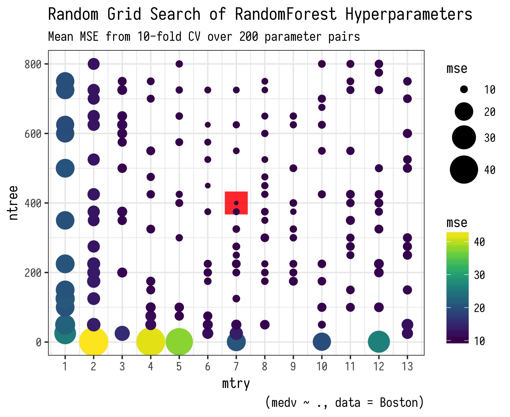
labs(title = "Random Grid Search of RandomForest Hyperparameters",
subtitle = paste0("Mean MSE from ", cv_folds, "-fold CV over ",
searches, " parameter pairs"),
caption = "(medv ~ ., data = Boston); Red square at minimum MSE") +
theme_bw() +
theme(
text = element_text(family = "Iosevka")
)

As noted in the warning above, I do not recommend running this on more than 50 or some hyperparameter pairs unless you plan to wait a while and have more than 16Gb of available ram. If you are doing real science here, its worth the wait, but not for a code example in a blog post! Below is a plot of running this for 200 hyperparameter pairs if you are curious.
Parallelize with future package!!!
Mapping over the rows of a tibble is an interesting way to execute a number of similar functions in sequence. However, since the evaluation of each hyperparameter pair is independent of each other, it makes the perfect scenario to parallelize the sequence. Fortunately, the future package by Henrik Bengtsson gives us the ability to easily modify the purrr::map() code to take advantage of a parallel backend. I don’t have the time or knowledge to give a formal introduction to the future package, but I can show you a quick way to use it. To read more about the future package check out this vignette
The core idea of the future package is that it allows you to write code that will be evaluated in the future; hence the name. It is a bit like a queuing system that can use a bunch of different methods to queue and execute your code in a synchronous or asynchronous sequence that takes advantage of available computational resources. I know I am not doing justice here! The main part of setting up your code is to choose a future::plan(). The plan is the method by which you plan to queue code and execute it as cores become available. The two plans that I have used are multisession and multiprocess. The former is available on all platforms and creates a bunch of background R sessions to take up the work. The latter is a bit more like traditional multicore parallelization and uses the current R session to execute everything. I will use multisession here.
library("future")
future::plan(multisession) # <- setup parallel
If you get even a little into the future intro vignette, you will see that there is a bit of new syntax used to setup code for parallel evaluation. Most notably is the %<-% assignment operator. However, since we are deploying this into an existing purrr::map() sequence, we will use a different approach to send functions to the queue. The code block below is nearly identical except for changes to the three lines with comments. The three main changes are:
- Start a new
mutate()call after the folds are created - The
map()function is now wrapped in afuture::future()call;~future::future(rf_helper(.x)) - Another new
mutate()call is made to collected the values from thefutureR sessions and continue on to the mse error extraction.
So that’s it! The hardest part was starting a mutate() call and the little but of syntax to wrap the function in the map() call into a future::future() call. Note, I use future::future() instead of just future() because I think being explicit about the package/environment is go, but either will do. Also, within the future() wrapped call to rf_helper() and future::value() I need to include the .x as the place holder for the data that is the first argument in the map() function; that is folds and model respectively.
model_fits <- seq_len(searches) %>%
  tibble(id    = .,
         ntree = sample(c(1,seq(25,max_trees,25)),length(id),replace = T),
         mtry  = sample(seq(1,ncol(data)-1,1),length(id),replace = T)) %>%
  nest(-id, .key = "params") %>%
  mutate(folds  = list(rsample::vfold_cv(data,cv_folds)),
### start new mutate()
         folds  = map2(folds, params, cv_helper)) %>%
### send rf_helper call to queue
  mutate(model  = map(folds, ~future::future(rf_helper(.x)))) %>%
### collect the values of rf_helper
  mutate(model  = map(model, ~future::value(.x)),
         mse    = map_dbl(model, MSE_helper))
After that fires off on all cylinders, the model_fits tibble is the same as the non-parallel version and the plot function is identical. I won’t guarantee that given your system, model, ramm that this will be faster; with randomforest memory is usually the bottleneck. However, when I did some tests across a few hundred hyperparameter evaluations, I saw a approximate 14% decrease in execution time.

So that’s it! Let your mind run wild about the sort of models/simulations/experiments that you can run in parallel while mapping across a table of values. The result is an incredibly readable and super compact data structure. There is something satisfying (or perhaps insane…) about completing an entire analysis from data ingest, clean-up, modeling, and inference in a short series of purrr::map() calls and then seeing the entire process stored in one table. A purrr-fect way to tidy up your code!

What a fantastic tutorial!
I saw a small typo, mutlidimensional.
LikeLiked by 1 person
Thanks Maëlle!
LikeLike