Execution Time of data.table vs dplyr

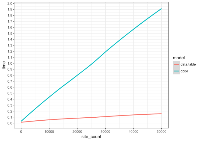
This code shows the difference in execution time and rate of execution time increase for an analysis function coded in two different approaches, 1) data.table, and 2) dplyr. This analysis is the result of working with this function and using profvis to optimize. The end result is that the data.table version is much faster across all simulations and scales much better than the dplyr version. Please read through and check out the profvis results linked in the list below.

Notes:

• The full code of this comparison can be found here
• I use profvis to profile the execution time of each function, the full results are here for dplyr and here for data.table
• I love dplyr and use it for everything. This is not intended as a critique, just some information on execution speed
• My use of dplyr may not be optimum and may be contributing to the speed issues
• the overall approach could also be optimized, but it represents a typical use-case balancing code clarity and function
• If you see a flaw or speed trap in any of the code, please let me know. Thanks.

Finding

Data.table approach is 0.124 seconds faster at 10 sites/events, is 0.922 seconds faster, at 25,000 sites/events, and is 1.735 seconds faster at 50,000 sites/events. For every 1000 sites/events added the data.table approach execution time increases by 0.0277 seconds; dplyr increases at a rate of 0.3765 seconds.

Functions

Below are the two versions of the same function.

The function being tested here computes the aoristic weight for a series of simulated data. What an aorsitc weight is really doesn’t have much to do with this post, but if you are interested, more information can be found here. This somewhat obscure function is useful here because it is an example of the sort of function that an analyst would have to code themselves and therefore run into the decision of using dplyr or data.table. Obviously, you could write this is C++ or do something else to optimize it if that was your priority. However, this is a more realistic comparison (IMHO), as much of an analyst’s time is spent balancing optimization versus getting-stuff-done.

note: there is a little weirdness with negative dates and start/end dates. This is because I started out with BCE dates and then switch to years BP dates to match another analysis. So, it is little bit of a hodge-podge in dealing with BCE and BP.s

data.table version

my_aorist_DT <- function(events, start.date = 0, end.date = 2000, bin.width = 100) {
  require(data.table)
  setDT(events)
  time_steps <- data.table(
    bin.no  = seq(1:(abs(end.date)/bin.width)),
    Start = seq(start.date,(end.date-bin.width), by = bin.width),
    End   = seq((start.date+bin.width),end.date, by = bin.width))
  setkey(time_steps, Start, End)
  overlap_names <- data.table::foverlaps(events, time_steps,
                                         type = "any", which = FALSE)
  overlap_names <- overlap_names[i.Start != End & i.End != Start]
  overlap_names[, duration := (i.End - i.Start)]
  overlap_names[, W := (bin.width / duration)]
  ov_sum <- overlap_names[, .(aorist = sum(W),
                              median_step_W = median(W),
                              site_count = .N), keyby=.(bin.no)]
  setkey(ov_sum, bin.no)
  setkey(time_steps, bin.no)
  ov_sum2 <- ov_sum[time_steps, nomatch = NA]
  ov_sum2[is.na(ov_sum2)] <- 0
  ov_sum2[, bin := paste0(Start, "-", End)]
  return(ov_sum2)
}

dplyr version

my_aorist_dplyr <- function(events, weight = 1, start.date = 0, end.date = 2000,
                      bin.width = 100, round_int = 4) {
  require(dplyr)
  require(data.table)
  time_steps <- data.frame(
    bin.no  = seq(1:(abs(end.date)/bin.width)),
    Start = seq(start.date,(end.date-bin.width), by = bin.width),
    End   = seq((start.date+bin.width),end.date, by = bin.width))
  setDT(time_steps)
  setDT(events)
  setkey(time_steps, Start, End)
  overlap_names <- data.table::foverlaps(events, time_steps,                                           type = "any", which = FALSE) %>%
    filter(i.Start != End & i.End != Start)
  aorist <- overlap_names %>%
    data.frame() %>%
    group_by(name) %>%
    mutate(site_count = n(),
           W = (bin.width / (i.End - i.Start)),
           W = round(W,round_int)) %>%
    arrange(name, bin.no) %>%
    group_by(bin.no) %>%
    summarise(aorist = sum(W),
              median_step_W = median(W),
              site_count = n()) %>%
    right_join(., time_steps, by = "bin.no") %>%
    replace_na(list(aorist = 0, site_count = 0, median_step_W = 0)) %>%
    mutate(bin = paste0(Start, "-", End)) %>%
    dplyr::select(bin, bin.no, aorist)
  return(aorist)
}

Simulation Loop

The simulation loop simply loops over the 1001 site/event counts in sim_site_count_seq. For each loop, both functions are executed and the time it takes to run each is recorded into the table below.

To see the full code for this list, check it out here.

	measure
site_count_min	10.000
site_count_max	50000.000
dplyr mean (seconds)	0.995
DT mean (seconds)	0.095
max difference (seconds)	1.981
min difference (seconds)	-0.002
mean difference (seconds)	0.900
mean RMSE	0.006

Plot results