Background Sampling & Variance in Logistic Regression Models

In preparing for a talk on Archaeological Predictive Modeling (APM) next week in Concord, NH I made some graphics to illustrate a point. A blog post is born.

Cutting to it… If you want to use logistic regression to build an APM you are using site locations as the positive class (site present) and some form of the environmental background as the negative class (site absent). How you conceptualize site absence is a bigger fish that I have time to fry here, but for the sake of conversation these models are taking random selections of 10 meter x 10 meter non-site cells to simulate the general environmental background. It is important to note that using the locations of surveys that failed to identify archaeology sites is often problematic because of location/selection bias, imperfect detection, or just lack of surveys. For these reasons, we need to make assumptions about how the background is represented. So making the assumptions that we often do raises one big problem:

How many samples are needed to adequately characterize the background?

Good question. The answer depends on many things, but chiefly it depends on how many site samples you have and how diverse your environment is. Use as many as possible? Problem is given that the occurrence of archaeological sites are typically low prevalence events on the landscape, the more background samples we use per site sample negatively effects our sample imbalance. Sites are already in the minority, so adding more background to get a better characterization creates a larger imbalance and wreaks havoc as we will see. Ok, so use a balanced number of background samples, 1:1? That would be nice for the imbalance issue, but the fewer samples, the less we are to accurately characterize any relatively diverse environment. Fine then, how about 3:1 background to site samples? Sounds like a pretty good choice, lets start with a simple model:

$\log\{\frac{p}{p-1}\}=\alpha+\beta_1*water+\beta_2*slope+\epsilon$

Simple logistic regression with site presence/absence as the response, distance to water (ed_h6) and a measure of slope variation (slp_32c) as the dependent variables, and epsilon is assumed to be normally distributed and iid (but its not, lets not kid ourselves). The plot below shows the response curves varying across each variable as the 0.05, 0.5, and 0.95 quantiles of the variable named in the upper panel. Pretty weak signal, but there is something here. Basically, the probability decreases mainly with increased slope variation and more subtly with distance from water. That fits ok with pre-contact settlement in this area; give or take. The second image shows how they effect probability together.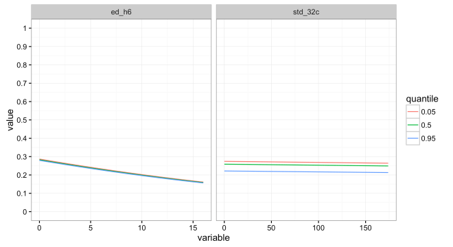 predict_by_quantile

probability_contour

Cool, models done. Nope. This outcome is based on a single draw of 597 background samples from a 3:1 balance for the 199 site location samples. What happens if we try again with another random sample of 597 background samples? All hell breaks loose! The gif below shows the response curve for the 0.05 quantile for distance to water over the range of slope variability for 100 different draws of 597 random background points. It is clear that taking a different sample may lead to a very different model outcome. Logically, this should not be shocking, but relying on a single relatively small random draw for a background sample is a rather defacto approach to APM. Unfortunately, simply taking a larger sample does not solve all our problems.

background_samples

The gif shows essentially the same as above, but varying across different ratios of background to site samples. Starting with 3:1 on the left and increasing to 20:1 on the right. As the ratio of background to sites increases, the variance between models decreases (less erratic fit lines), but the overall increased imbalance of background to sites leads to reduced overall probability. The lower variance is a good thing, but the overall lower probability is not.

Background samples by mutliplier

Ways to address these competing issues include finding the right ratio balance, modeling techniques that address highly-imbalanced data, bootstrap sampling of the background, or model averaging; in addition to different algorithms and model specifications. Hopefully this illustrates the danger of relying on a single random draw to represent site-absence locations and the utility of criticizing you model results against multiple draws.

Notes:

The top two graphics are not actually the simple logistic regression example. These are drawn from a Bayesian HMC GLM with priors $\mathcal{N}(0, 1)$ , but the response is pretty much the same. The uncertainty of 1000 posterior draws of a single 3:1 background sample is presented here:
Clearly, the effect of ed_h6 and std_32c on presence/absence given these assumptions and mode is not great. However, these two variables are well ingrained in temperate area settlement theory and recognizable to any archaeologists. They make a good example for discussion.